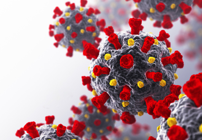
Credit: iStock
Since early in the pandemic, when genomic material of SARS-CoV-2 (the virus that causes Covid-19) had been detected in air samples and well-documented superspreading events were reported, there was an implication of long-range airborne transmission. Accordingly, CIBSE advised increasing ventilation airflows as much as reasonably possible, taking into account occupant comfort and energy use concerns.
However, it is impossible to calculate a universal flowrate that would lead to a constant, universal reduction in transmission risk – not least because the emission rate of viable virion from an infector varies over the time since infection. People also have different emission rates, ranging over several orders of magnitude. Equally, there is no knowledge on dose-response characteristics of SARS-CoV-2 in humans.
Output numbers from the model are for illustration only, but are useful to observe trends and understand absolute magnitudes
A further complication is that virions entrained in aerosols have additional removal mechanisms – biological decay and deposition – that are space -volume dependent (see ‘Why space volume matters,’ CIBSE Journal, June 2021). To overcome some of these uncertainties, Jones et al developed a relative risk index, which enables the analysis of the relative risk of long-range aerosol transmission between a reference and comparator of an indoor scenario if the same infector is present in both scenarios (bit.ly/CJNov22CI1).
This method has been adopted by the CIBSE air cleaning guidance as a means of establishing relative risk reductions from different ventilation and filtration strategies (see ‘A novel approach: air cleaning devices,’ CIBSE Journal, September 2021).
However, the probability of the presence of infected people and the number of susceptible people increases with the number of occupants in a scenario, so population-level risks are different. We have recently published a novel framework methodology to help determine this difference and give an insight into the absolute magnitudes of risk reduction.1
The problem
Assume an office space has 30m3 of space per person and is ventilated at 10l/s/person; would you rather spend eight hours in a five-person office or a 50-person office? If you were to share either office with a single infector then, from a personal risk perspective, the 50-person office would be lower risk.
This is because the virion removal equivalent flowrates – in l/s (ventilation, deposition, bio decay) – are 10 times larger in the 50-person office, leading to a 10-fold lower concentration of virus in the air compared with the five-person office. The inhaled dose and relative exposure index will be 10-times smaller in the 50-person office.
But what about population risk? There are 10-times more people in the 50-person office, so the presence of an infector is more likely – and if an infector is present, there are more susceptible people sharing the scenario to infect.
The probability of sharing a scenario with an infector is dependent on the community infection rate (CIR) – in other words, what proportion of the whole population is infected and could potentially share the space. If we assume 1:100 people is infected, what is the most likely number of infected people in the 50-person and five-person office?
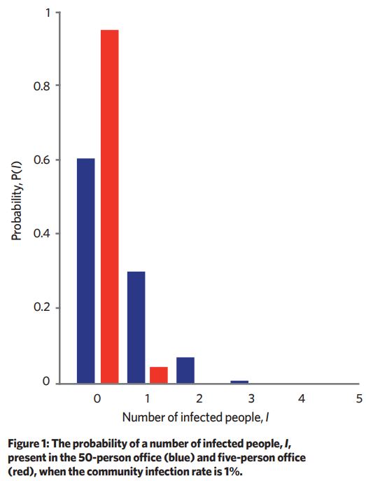
We can think of this problem like pulling balls from a bag – given a bag of 990 red balls and 10 white balls, in random draws of 50 balls the most common number of white balls drawn would be zero. Using combination theory, we can predict the most likely number of infectors in a given scenario if we have the scenario occupancy and the CIR (see Figure 1).
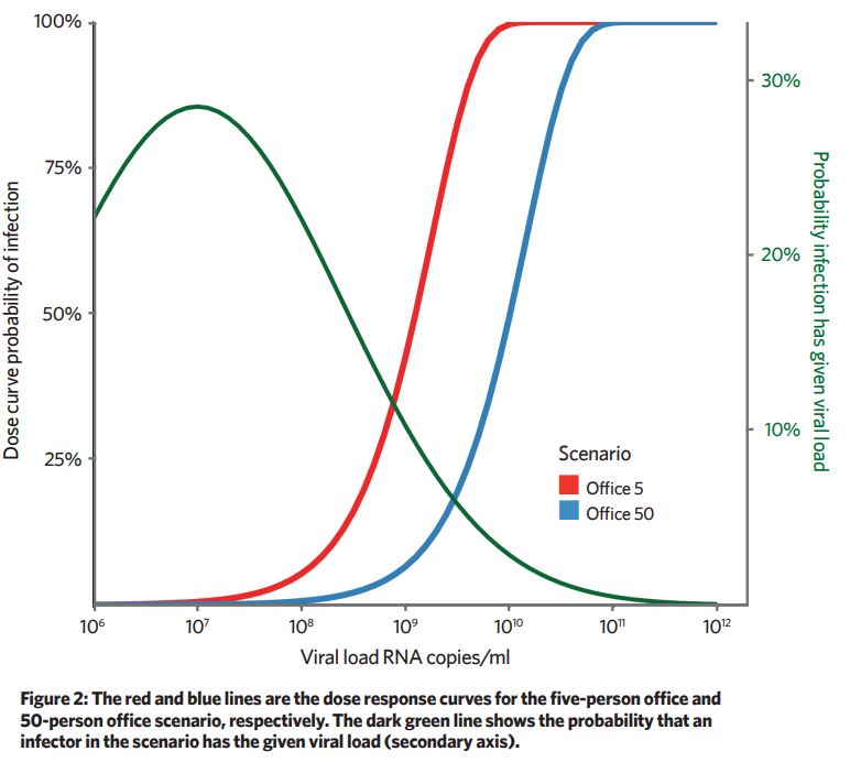
Even if there is an infector present, the viral load of the infector will vary by several orders of magnitude. Viral load of infector is proportional to the amount of virus they can emit into the air. The more virus exhaled, the greater the concentration of virus in the air, which increases the inhaled dose of susceptible occupants.
A dose curve is used to predict what proportion of the susceptible occupants would be infected for a given dose. Because the removal mechanisms are 10-times greater in the 50-person office, the viral emission rate needs to be approximately 10-times larger to give the same probability of infection.
Increasing removal mechanisms – for example, ventilation and filtration – has the effect of shifting the dose curve to the right. For low viral-load infectors, the probability of infection is near zero, and for high viral infectors the dose is near 100% (Figure 2).
We have to make some assumptions on viral load to viral emission rate and dose response for these calculations (the limitations are considered in the paper), so output numbers from the model are for illustration only, but are useful to observe trends and understand absolute magnitudes.
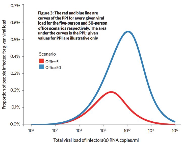
We can approximately calculate the proportion of a given population, distributed in either five-person or 50-person offices, infected for every given viral load.
The proportion of people infected (PPI) ≈ proportion of people susceptible x infection probability x probability the infector has the given viral load. This is calculated for each viral load and the resulting graph gives the total proportion of people infected as the area under the graph (Figure 3).
For the given assumptions, at a population scale, the transmission risk in a 50-person office is about three-times higher. This isn’t a magnitude that would suggest there is advantage in dividing a 50-person office into 10 cellular five-person offices, but this method could help explore which scenarios would lead to better reductions in long-range airborne transmission.
Here, for example, improving a poorly ventilated 50-person office would lead to a greater PPI reduction than improving a poorly ventilated five-person office, so could be useful when scheduling which scenarios within a portfolio should be targeted first for improvement.
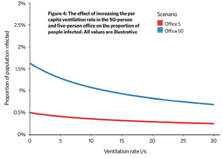
We don’t know absolute values, but it is useful to look at trends in PPI when we adjust various parameters. Increasing ventilation of poorly ventilated spaces reduces PPI more than increasing ventilation in an already well-ventilated space (Figure 4). Reducing occupancy or increasing space volume per person also reduce the PPI.
This framework also shows that, in many scenarios, there are no infectors or an infector with a viral load so low that they don’t emit enough virus to lead to long-range infection of susceptible people. Then, ventilation has little effect. If an infector has a very high viral load, ventilation can’t reduce infection rates much because the concentration in the air is too high.
A ‘Goldilocks’ zone exists between these two extremes where the situation is ‘just right’ for ventilation to have an effect. Then, improving poorly vented spaces has the greatest effect on the reduction of the long-range transmission risk. At all times, the concentration of virus in air is highest in the exhaled puff, so the ‘coffee breath’ zone (close contact) is where exposure risk is greatest.
About the author
Chris Iddon MCIBSE is chair of the CIBSE Natural Ventilation special interest group
References:
- A population framework for predicting the proportion of people infected by the far-field airborne transmission of SARS-CoV-2 indoors. Building Environment, August 2022 bit.ly/CJNov22C1 There is an open version at bit.ly/CJNov22C2