Acoustic analysis for building services becomes more demanding with novel forms of passive and active environmental systems. However, the basic principles of acoustics do not change – it is simply their application. The impact of ‘sound’ in buildings can be airborne and so heard directly by the ear, or passed through surfaces so that it is felt as vibrations. Whether that sound is treated as ‘noise’ will depend on circumstance – a hum from a fan may be reassuring sound for the facilities manager but could be an intrusive noise to the office worker. This CPD will explain the underlying acoustic terminology that provides a basis for setting the standards and maintaining airborne noise at an acceptable level appropriate to the application.
A very simple (pure tone) sound will travel through the air as shown in Figure 1.
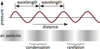
Figure 1: A representation of a simple pure tone travelling through air
The distance between the ripples of successive high pressure points is known as the wavelength, λ (m), of the sound and the frequency, ƒ (Hz), is the number of times that the pressure peaks per second at a particular point. The pressure ‘wave’ will travel through the air at speed c (m·s-1), varying the pressure at each point somewhere between maximum and minimum pressure; this range is twice the amplitude, P (Pa). Wavelength and frequency are related by λ = c / ƒ.
The sound travelling in the air (by successive collisions of molecules) will have a velocity of about 343 metres in one second; this can be determined from the simplified relationship c = 20√T, where T is the absolute temperature of the air, K. A person would ‘hear’ the sound as the tympanic membrane in their ear moves in and out, as the sound ‘wave’ changes the pressure on the outside of the ear. The sound will also pass through solid materials, albeit much faster, as the molecules are more densely packed (for example, through brick at about 3,000 m/s). Whether passing through the air or through a solid, there will be some attenuation of the sound’s strength as it travels, since some of the energy will be scattered and absorbed by the material (and some converted to heat). And, of course, for sound to travel there does need to be a liquid, gas or solid, so that there is a transfer of pressure variations – the more densely packed molecules will transfer sound more effectively.
Sound is related to a cycling of pressures, typically illustrated by a sinusoidal wave (as in Figure 2). This form of representation is a convenience that illustrates the pressure variations with time at a particular point; actually, the sound is a longitudinal wave (moving in all directions), with areas of high and low pressure (known as ‘compressions’ and ‘rarefactions’, as in Figure 1) that ‘travel’ like the ripples on a pond, where the wave moves (losing intensity as it proceeds) without any flow of water. A ‘pure tone’ can be represented simply in terms of its frequency, ƒ1, with its strength represented by the height of the line (as in Figure 2).
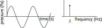
Figure 2: Simple pure tone resolved into a single frequency and rms pressure
More complex sounds can be resolved into a number of different frequencies (each with their own amplitudes) that can be represented as combining together to make a sound. For example, the relatively simple waveform in Figure 3 could be resolved into three frequencies, each with their own strength.
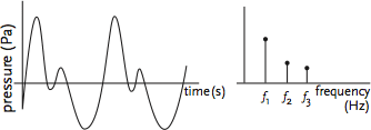
Figure 3: A slightly more complex sound
In the real world, there are sounds that are said to be ‘continuous’, such as that shown in Figure 4. This is made up of many frequencies that make it practically impossible to break it up into discrete pure tones. In order to represent this type of sound, which is very common, the frequencies are measured in ‘bands’ (similar concept to ‘bins’ in external temperature assessments).Thesebands (that may be ‘octave’ or ‘1/3 octave’ bands) more readily visualise the characteristic of the sound by losing the detail of individual frequencies. The use of octave band analysis must be employed with care, since there may be peaks of frequencies that occur within the band that will be ‘levelled out’ by the averaging effect within a complete band.
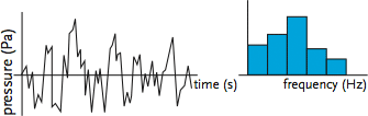
Figure 4: Octave band frequency analysis
The actual strength of a particular sound felt by the ear is related to the fluctuations of sound pressure (Pa) reaching the ear. The strength of the source itself is determined by the sound energy output, known as sound power (W), and for a piece of equipment would typically be assessed in a test chamber. The sound power is an attribute of the item that is generating the sound (such as a fan), and is normally assumed constant for a piece of equipment regardless of location. However, the sound pressure is related to the position of the listener relative to the sound source, and is affected by the distance from the source and by the acoustic surroundings.
The range of sound powers (and resulting sound pressures) is very large – from a whisper at 10-9 W through to a space rocket at 106 W. Human sound perception does not vary linearly with the intensity – intensity being the amount of sound power per unit area (W·m-2) – and the listener would not perceive a 1015-fold difference between the whisper and a rocket but relate it to their threshold of hearing in a way that is similar to a logarithmic scale. So, to better represent the ear’s response to sound, and to allow the manipulation of these numerically disparate values, logarithms are typically used.
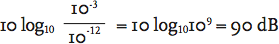
The threshold of hearing corresponds to a pressure variation less than a trillionth of atmospheric pressure, and to reflect this, a reference sound power (or datum) is taken as 10-12 W (1 pW), and the sound power level is calculated relative to this.
sound power level, LW =
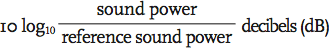
The value of the ‘Bel’ is given by the log (to base 10) of the ratio of two quantities – in this case, two sound powers. The ‘decibel’ is a tenth of a Bel (hence the multiplier ‘10’ in the equation) and provides a more usable scale – the Bel is not used in acoustics.
So, for example, if a fan has a sound power of 0.001 W, the sound power level would be
As the ear responds to sound intensity I, where I = p2/ρc and ρ is the air density (kg·m-3) and c is the speed of sound (m·s-1), the sound pressure level uses a ratio of the square of the sound pressure to provide a usable and relevant metric for sound pressure. So,
sound pressure level, LP =
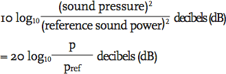
and Pref is the pressure at the lower end of human audibility 2 x 10⁻⁵ Pa (or 20 μPa)
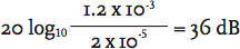
So, for example, in the middle of a library, if the sound pressure is 1.2 x 10⁻³ Pa, the sound pressure level, LP =
A 3 dB change in sound pressure level is just noticeable, a 5 dB change clearly noticeable, and a 10 dB change is twice (or half ) as loud.
If there is more than one source of sound in a room, then the sound pressure level may be added together by first converting back to the square of sound pressure, adding and then reconverting back to dB or, rather more easily (but approximately), the table below may be used to add the different sources together.
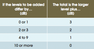
Figure 5: Approximate method of adding dB sound sources together
So, for example, if one source has a sound pressure level of 45 dB and another 46 dB, the difference is 1 dB, and so the overall sound pressure level is (46 + 3) = 49 dB.
The ear does not respond equally to all frequencies. This appreciation of loudness is reflected in the phon scale, as shown in Figure 6. For example, the 50 phon contour shows values of LP for other frequencies that are perceived equally loud as 50 dB at 1,000 Hz, and looking at a frequency of 100 Hz, a sound pressure level of nearly 60 dB will have the same perceived loudness as 50 dB at 1,000 Hz.
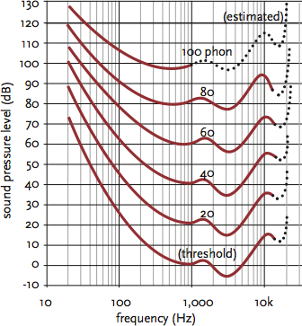
Figure 6: Phon – equal loudness contours
The curves indicate that generally low (or very high) frequency sounds need to have a greater sound pressure level to be perceived as loud as mid-range frequencies. These curves were developed from original experiments in the 1930s and have recently been altered in ISO2261, notably with the shift of the most sensitive frequency from 4 kHz to 3.5 kHz and amended to be less sensitive at frequencies below 1 kHz.
A young person may be able to hear sounds from 20 Hz to around 20 kHz. Below this, frequencies are known as infrasound; higher than this normal hearing range is termed ultrasound. In the hearing range, perceived loudness is critical in the assessment of the acoustic environment, as this will influence the design and operation of systems so that they do not adversely affect people.
The value of sound pressure level may be weighted in terms of the ear’s ability to hear them. There are several different methods of weighting that may be applied, but for the relatively low intensities within buildings, weighting network A, or dBA, is commonly used. This weighting practically simulates the 40 phon contour by attenuating the lower frequencies and clipping the highest frequencies. Where there is predominantly low frequency noise, dBA may well underestimate the apparent loudness. However, this weighting is widely used to determine noise levels for building services applications.
For example, a series of octave band sound pressure levels have been measured in a room (as in Figure 7), and the dBA weightings are applied to determine the total A-weighted sound level. Noise weightings B and C relate to higher phon levels and are not often used in building services applications – they take greater account of lower frequencies.
.png)
Figure 7: Example A-weighting of octave band sound pressure levels
When using a sound meter, the reading is normally directly in dBA, and there is no need to convert; indeed, it is the more expensive instrumentation that allows an octave band analysis (or even a ‘third octave band’ where greater discrimination is required). If octave band frequency analysis is available, then the data may be transferred onto a set of noise criteria (NC) curves or noise rating (NR) curves. These are useful, as they not only give a value that can be compared to design standards but will also help identify frequency bands that may cause potential problems.
The NC curves are of American origin and were originally designed for use in office applications to assess the noise. The NR curves are European, designed for general ‘environmental’ application, and are more tolerant of the lower frequency noise but less tolerant of high frequencies. Figure 8 provides an NR value for the spectrum used to determine 51 dBA above – this provides an NR47. dBA may be approximately translated into NC or NR by taking 5 away from the dBA level.
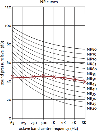
Figure 8: Noise rating curves
When the sound level is measured, it will be (as set on the measuring device) ‘fast’ to show quickly varying noise, ‘slow’ to dampen out variations and give a more consistent reading, or ‘continuous’ to ‘average’ out the sound over an extended time period. Continuous ‘equivalent’ dBA is typically abbreviated to LAeq and is widely used to record environmental noise.
A future CPD will consider the application of these acoustic concepts to buildings and systems.
© Tim Dwyer 2012
Further reading:
CIBSE Guide B5: Noise and Vibration Control for HVCA, 2002.
References
- ISO226:2003Acoustics–Normalequal- loudness-level contours.