To provide reliable forecasting for energy costs and associated carbon emissions in a residential heat pump retrofit, it is important to understand the building thermal energy performance of the dwelling. London South Bank University (LSBU) is working with partners Parity Projects, RetrofitWorks, ICAX and Cambridge Energy Solutions on a Heat Pump Ready Programme Stream 2 project1, funded by the Department for Energy Security and Net Zero, that aims to provide tools that characterise building thermal energy performance.
The LSBU research uses a degree-day approach based on CIBSE Technical Memorandum (TM) 412, while Parity Projects is exploring Reduced Data SAP-related methods. Both models ultimately want to be able to show whether a heat pump is performing as expected, and whether under-performance can be explained in terms of system deficiencies, weather anomalies, or user behaviour.
The project has installed remote-monitoring systems into 18 houses – mainly older detached properties – with a target of 40 houses to be monitored by the end of the project. Each house has temperature sensors in selected rooms (typically four or five), heat meters for space heating and hot water (where appropriate), and gas and electricity data collection. Weather data is collected via dedicated local weather stations or from commercial sources of local weather.
TM41 describes a degree-day-based approach to estimating and monitoring space heating energy in buildings. It incorporates building heat loss coefficient, building thermal capacity and casual gains – together with operational factors such as occupancy profiles and control strategies – to capture quasi-dynamic energy performance against external temperature conditions. The complexity of energy modelling is reduced while a degree of mathematical rigour is retained. It modifies the classical degree-day approach by incorporating daily mean internal temperatures and casual heat gains into the degree-day calculation, to give building-specific base temperatures. The degree-day values can be used for performance measurement or future energy estimation – the former for building characterisation, the latter for energy use predictions.
This project examines how well the method works at different timescales – daily, weekly and monthly – and its accuracy using the high-quality data sets from the monitoring process.
Theory and method
Daily degree-days are the sum of the temperature difference between indoor base temperature and the hourly outdoor temperatures:
Dd=Σ(θb – θo,h) Δt
Where the base temperature, θb, is calculated from
θb = θi – QG/HLC
Where θi and QG are the mean daily internal temperature and mean daily gains respectively (kW), and HLC is the heat loss coefficient (kW.K-1; including both fabric and infiltration components).
Ε =24. HLC. Dd/η
Where E is the energy consumed for space heating (kWh) and η is the system efficiency (or coefficient of performance (COP) in the case of a heat pump). E can be plotted against Dd to analyse the energy performance of an existing building. In theory, the slope of a regression line of E v Dd is equal to the term 24.HLC/η.
This principle can be used to estimate the heat loss coefficient of a building and/or the system efficiency. The HLC used to generate the base temperature can be adjusted until it agrees with the slope of the regression line. This can be a far more reliable way to determine the actual heat loss characteristic of a building than from a physical survey. However, this principle only holds true if the correct base temperature is used in calculating degree-days, which will depend on knowledge of actual gains into the space. The research questions that arise are:
- What is the minimum amount of sensor deployment and data collection required?
- Which timeframe is most appropriate (daily, weekly or monthly) in terms of accuracy and data handling?
- Can the regressions be used to identify system-, weather- and behaviour-based anomalies?
Effect of timeframe
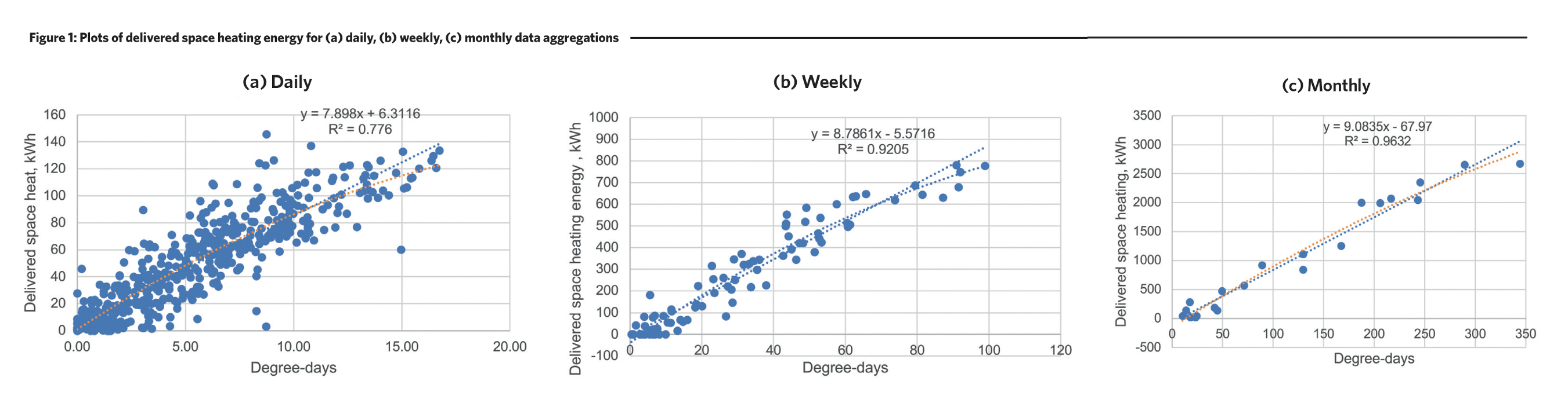
There are a number of ways to examine timeframe, particularly whether degree-days should be calculated to daily-varying base temperatures or whether longer-term averages can be used. In theory, the more fine-grained the better, but, in practical terms, long-term averages are easier to use because they require less granular data. The full paper examines this in more detail, and the example below shows one case where daily base temperatures are used for all timeframes. The example shows a detached house heated with a gas-fired combi boiler. Delivered space heating energy (from the heat-metered boiler output) is plotted against degree-days for daily, weekly and monthly timeframes. Note that the slope of this line is directly related to the heat loss coefficient (HLC=slope/24 kW.K-1). Two observations can be made between timeframes:
- The scatter reduces as the data is aggregated into longer timeframes and the R2 value increases markedly. Outliers at the daily level tend to disappear, which, in this case, can be explained in part by short periods where the system was switched off, but then took some days to warm the building back up. Losing these outliers can mean losing operational insights.
- The slope of the regression lines increases as the timeframe gets larger (and the intercept, which in theory should be 0, reduces). This is a trend across all buildings analysed to date, and is a characteristic of linear regression that needs to be fully understood. The current working hypothesis is that the daily timeframe gives the most reliable estimate of the heat loss coefficient because it contains more information about gain and internal temperature variations.
Case study – heat pump retrofit replacing oil boiler
The case study house has a 18th-century core with some additions and upgrades, and cavity-wall insulation and double glazing. It originally had oil-fired central heating, which was replaced with an 11kW air source heat pump. An in-line oil flow meter was fitted to the boiler just over one month before the heat pump installation. Prior to that, oil usage was measured from a 10-step oil gauge and quantities of bulk oil deliveries.
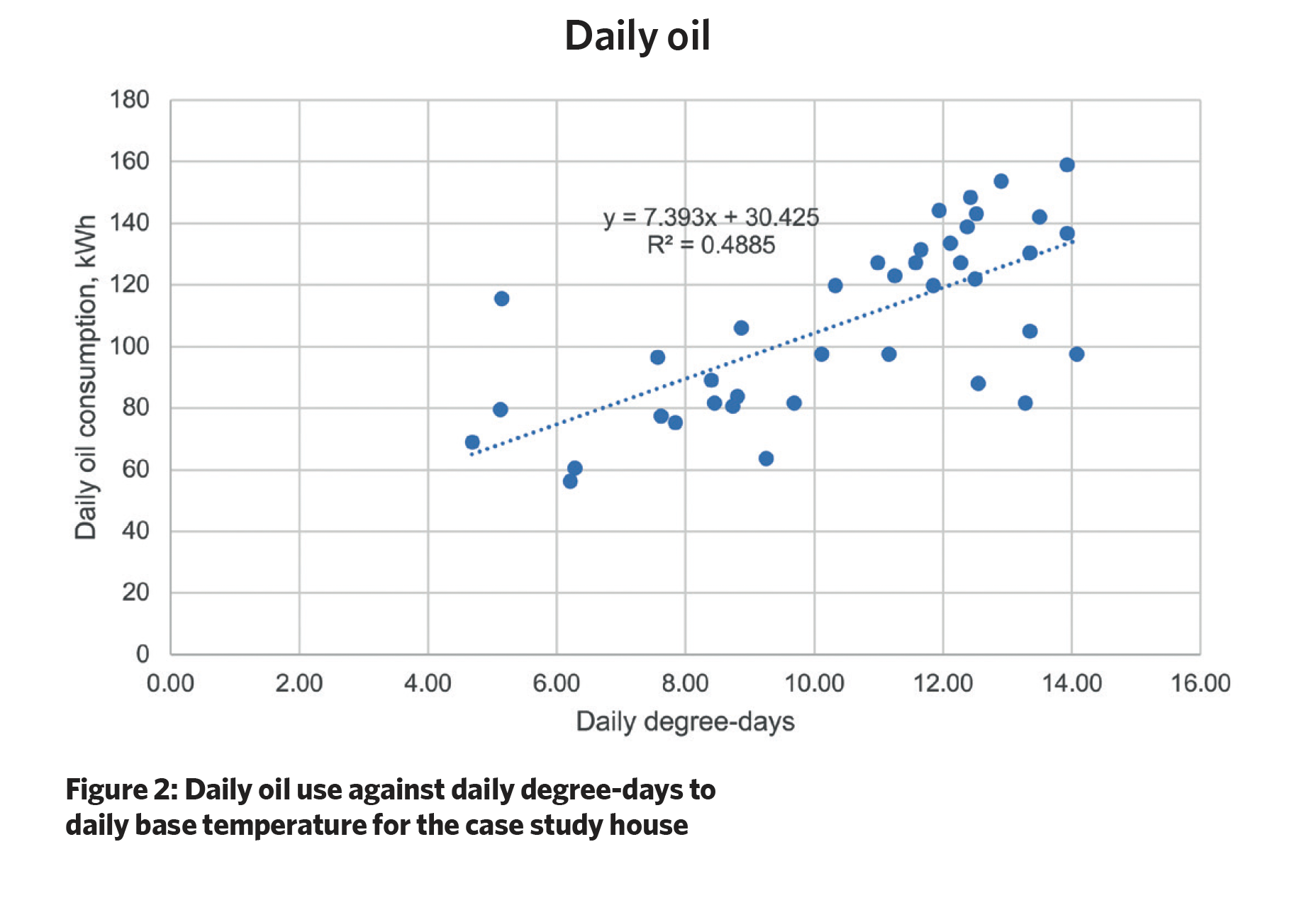
Figure 2 shows 39 days of oil meter data against daily degree-days to daily base temperatures. The R2 value is poor, and the slope (together with an assumed boiler efficiency of 0.85) indicates an HLC of around 0.26kW.K-1. This is lower than the surveyed estimate of 0.36kW.K-1. The intercept of 30.4kWh per day is high given that daily domestic hot water energy from summer use has been shown to be around 21kWh per day. Note that an analysis using bulk oil delivery returns an HLC of 0.346kW.K-1, considerably closer to the calculated value. This example indicates the difficulty of obtaining reliable baseline data from oil boiler installations, even if in-line meters are fitted (which is rare).
The heat pump was installed in March 2023, with integral electricity and heat metering. Figure 3 shows daily delivered space heating against daily degree-day to daily base temperatures for one entire heating season. The regression optimisation shows a slope of 8.88kWh per Dd, or 0.37kW.K-1, which is 7% higher than the previous oil regime analysis. The relationship is markedly better than for the oil boiler, indicating that the heat pump system employs a better control regime. Many of the outliers above the line can be shown to be because of weather events (in this case high winds from the south).
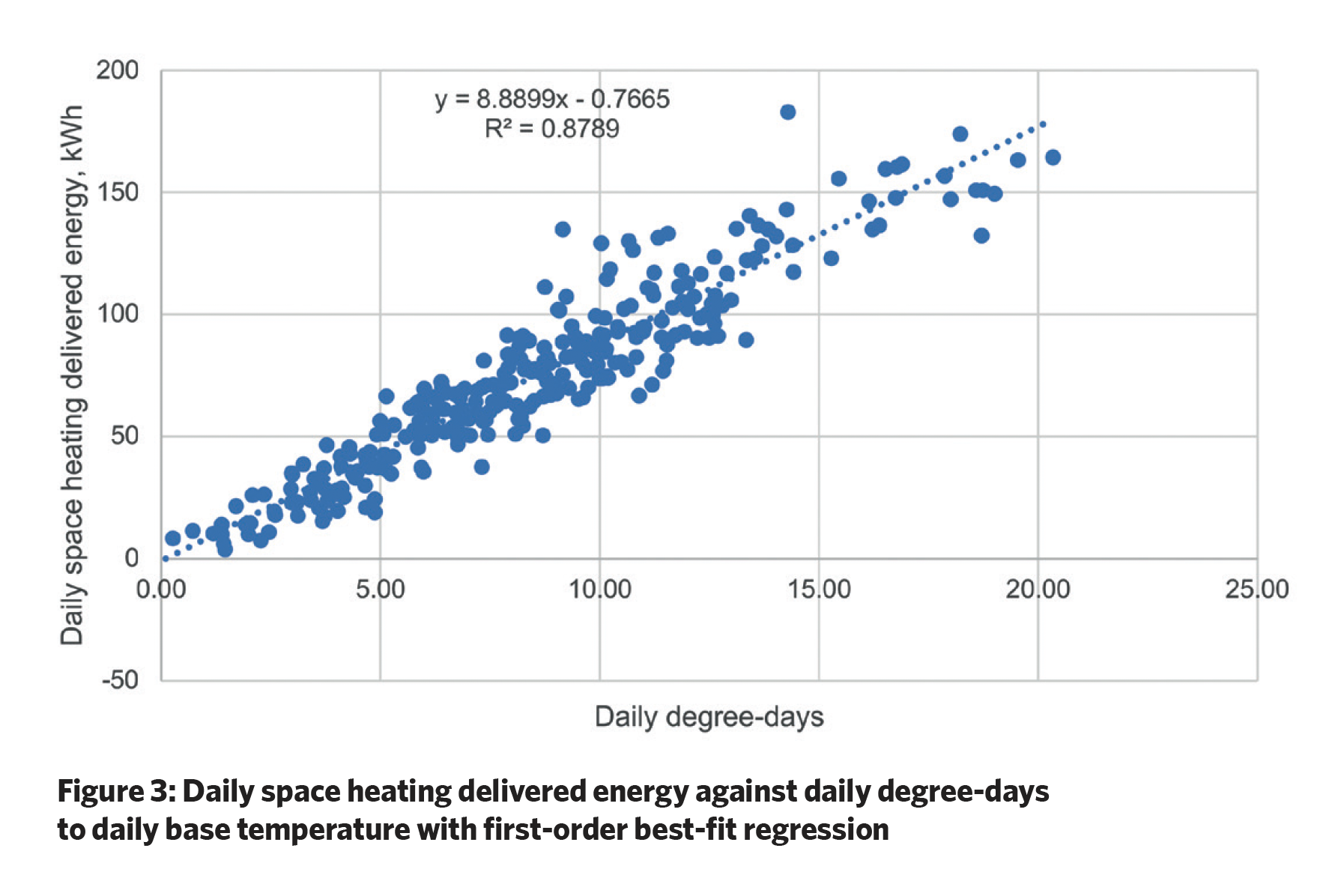
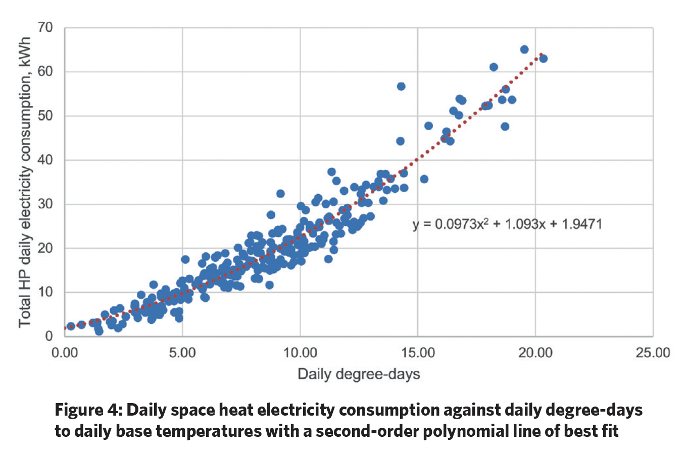
Figure 4 shows the daily electricity used by the heat pump for space heating. It is apparent that a simple linear regression (straight line relationship) is not sufficient here because of the large variation in COP across the heating season (possibly up to +/-30%), particularly in colder weather. A second-order polynomial is shown to be a good fit.
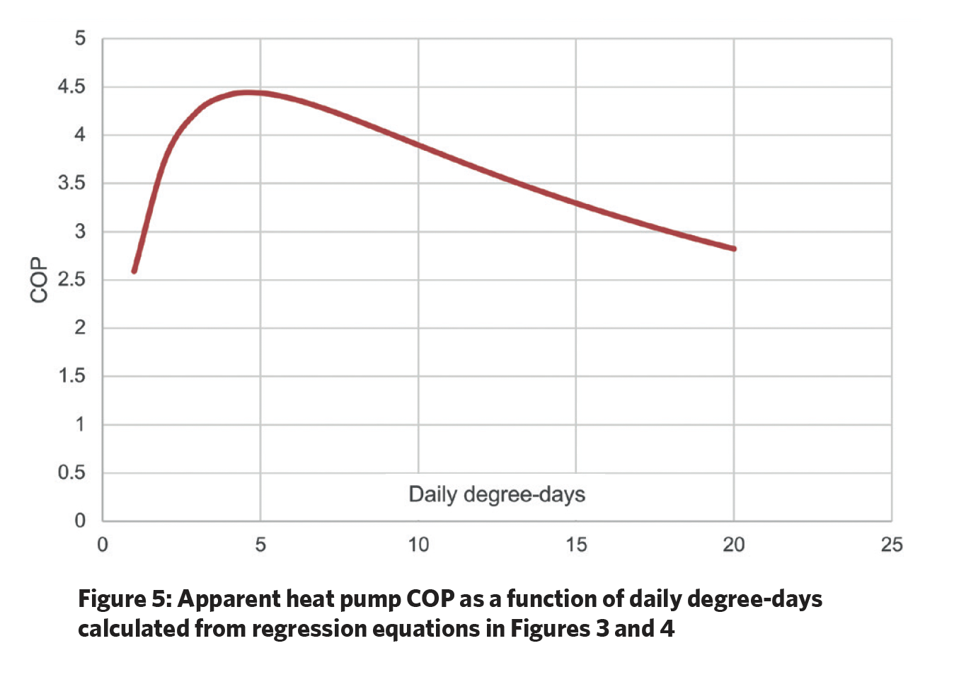
The regression equations for Figures 3 and 4 respectively can be used to develop a plot of expected heat pump COP for a given value of daily degree-days, as shown in Figure 5. This can be used to monitor the heat pump performance and identify system faults, or control anomalies by comparing with daily COPs in real time.
The preliminary results show how a TM41 degree-day approach can be used to characterise the thermal energy performance of a house, and form the basis of performance monitoring and anomaly identification. The next step in the research is to refine the predictive model for heat pump retrofits and validate the method using the range of properties being monitored in this study. The aim is to develop a set of rules by which regression models can be used to identify and explain system failures, user actions, or unusual weather events.
It is important that energy forecasts and performance monitoring methods are reliable and understandable to the householder, particularly where performance guarantees are in place. High levels of trust will be required where retrofit financing is funded through loans or operational savings and underpinned by such guarantees.
About the author
Tony Day FCIBSE is an energy research consultant
- This paper was presented at the 2024 Technical Symposium
References:
- Heat pump-ready programme: Stream 2 projects, Department for Energy Security and Net Zero, viewed 20 November 2023,
bit.ly/3QQP6gm - TM 41 Degree-days: Theory and practice, CIBSE, 2006 bit.ly/44QzwXS