The cooling of buildings accounts for 20% of electricity use worldwide, a figure that is projected to triple by 2050. As demand for data centres increases and global temperatures climb, the chiller market is projected to grow from $10.3bn in 2024 to $13.4bn by 2030.
A major driver of this increased energy consumption is the shift in data-centre cooling. The microchips used for artificial intelligence processing are pushing past the limits of traditional air cooling, with power demands expected to exceed 700W per chip by the end of 2025. Many of the facilities that were once cooled by direct-air cooling will soon require the generation of chilled water on site to facilitate direct-liquid cooling. (For more about the demands of data centres, see ‘Power struggle’, CIBSE Journal, April 2025.)
With the increased demand for cooling, and the urgency to reduce carbon emissions, predicting chiller energy consumption accurately has never been more important.
Early in the design process, engineers typically rely on the seasonal energy efficiency ratio (SEER) metric to estimate annual energy consumption of air cooled chillers. While useful for snapshot comparisons between machines, using SEER for this purpose is limited in its scope. It fails to account for basic factors such as hot exhaust recirculation and how numerous chillers will be staged when operating in tandem – and, therefore, how long each machine could operate in ‘free cooling’ mode. As a result, engineers risk miscalculating energy consumption and making sub-optimal equipment choices, which will have a real-world impact on a building’s energy use.
Life cycle carbon and energy modelling for optimal choice of chillers presents a simple and effective alternative model that can be used early in the design process to more accurately predict energy consumption. By using the linear average method, combined with a small amount of additional data from the manufacturer, engineers can map chiller performance across all external conditions and part-load scenarios, allowing for more in-depth analysis.
Linear average method
The proposed method for modelling gaps in the data is the linear average method. This is a two-step method that fully completes the gaps in the climatic information at 25%, 50%, 75% and 100% loading before modelling the gaps in the part-loading data. Manufacturers would need to provide performance data for various ambient conditions at 100%, 75%, 50% and 25% load. This would aim to capture the energy consumed by the fans, compressor and chiller circulating pumps. Some manufacturers may provide comprehensive data across all ambient conditions, while others might only be able to supply data at intervals, such as every 5K. Figure 1 shows how the energy efficiency ratio (EER) varies with ambient and part-loading conditions. The goal of the method is to accurately indicate the chillers’ efficiency during any of these.
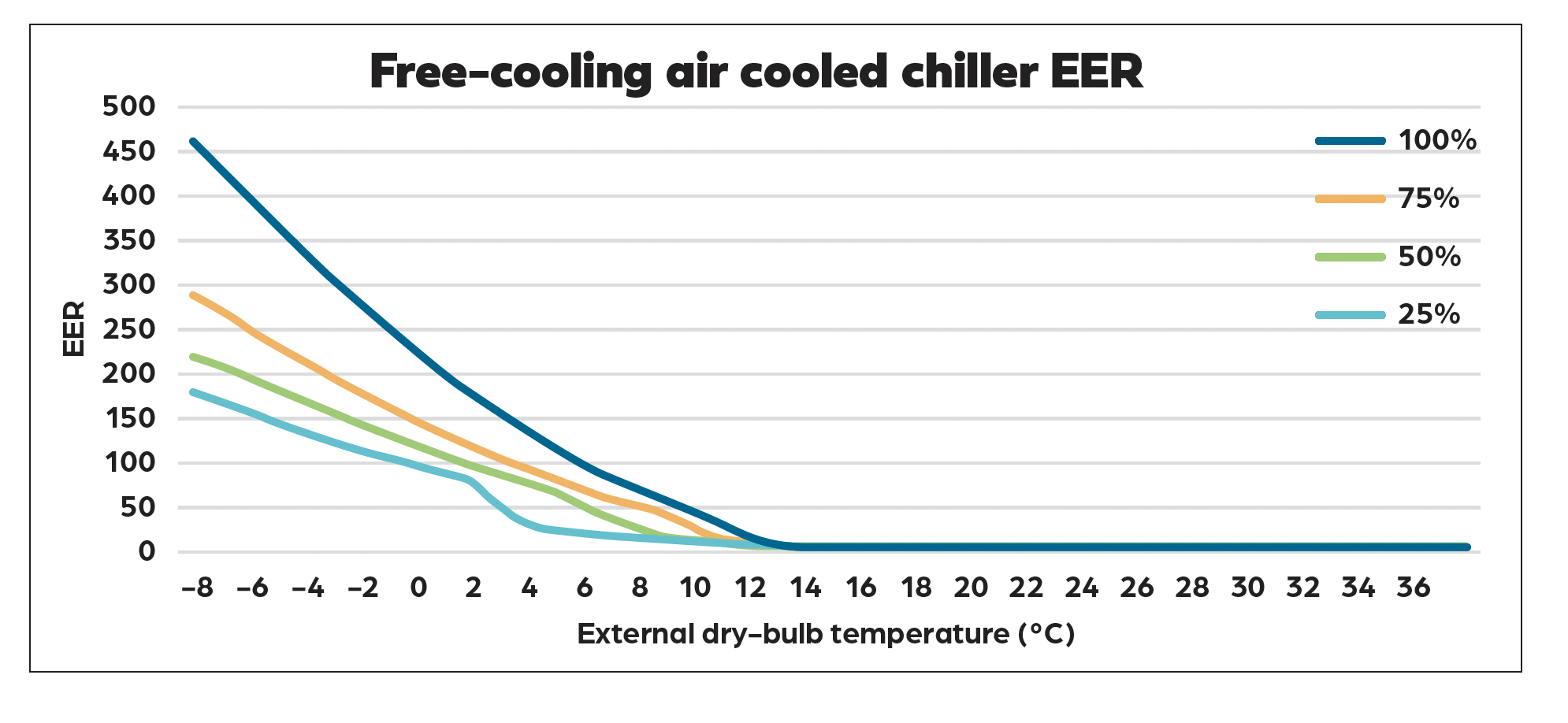
Figure 1: Example of true FC-ACC EER performance varying with temperature and part-loading
Modelling gaps in climate performance data
Figure 2 illustrates a method for estimating chiller efficiency (EER) when only two performance data points are available – in this case, at -5°C and 0°C external dry-bulb temperature. The actual performance curve, shown as the orange line, is derived from known EER values across the full temperature range and serves as a benchmark.
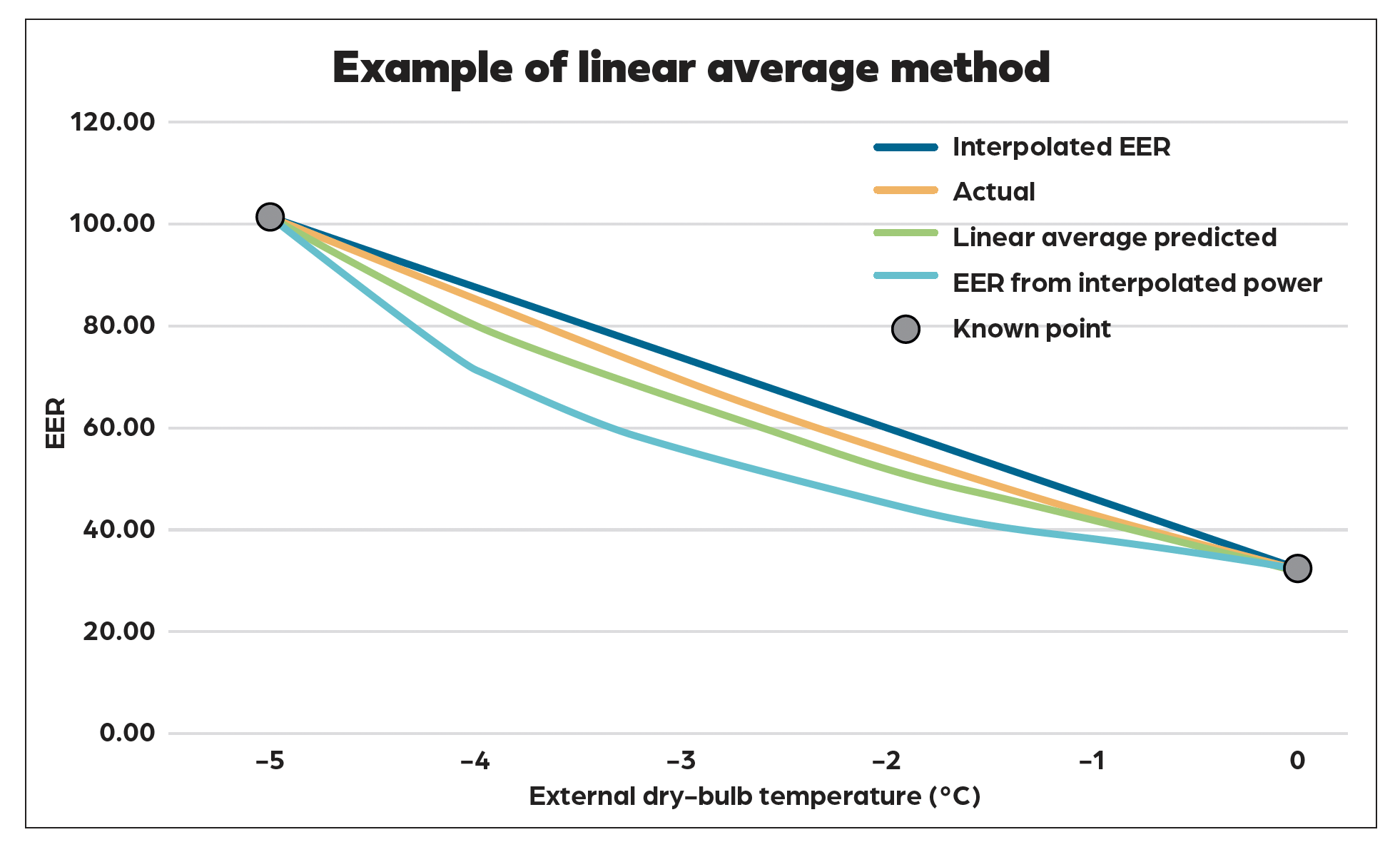
Figure 2: Actual and linear average predicted chiller EER between 0°C and 5°C
The first approach applies simple linear interpolation between the two known EER values generating the straight ‘Interpolated EER’ line (blue). This method tends to overestimate actual performance, however, because the true EER profile is typically convex – meaning that EER declines more rapidly than a straight-line assumption suggests. As a result, the linear interpolation is above actual performance curve.
An alternative approach involves interpolating power consumption rather than EER directly. Assuming constant cooling output, interpolated power values can be used to calculate estimated EER values, resulting in the ‘EER from interpolated power’ line (light blue). This method reflects a more realistic curvature in the performance profile, but tends to underestimate actual EER values.
To improve accuracy, a third method takes the average of the EER values produced by the two previous approaches. This produces the ‘Linear average predicted’ line (green), which is a much closer approximation to the actual EER curve than either method on its own and crucially does not overestimate the EER.
The example shown in Figure 2 examines just two points; the method is then applied between all known data points for a particular part-loading condition and shown in Figure 3 as the ‘linear average predicted’.
The advantage of this method is that it is very simple to implement in a spreadsheet. It is also robust when applied to a small dataset, as demonstrated in Figure 3 with nine data points for a given part-loading curve. A disadvantage of the method is that, with a very small dataset, it struggles to predict the large fall-off in performance when switching from full free cooling to mixed mode. By adding in this specific point, the issue can be alleviated, and its impact can be observed in Figure 3. It is recommended that this point is included in the initial dataset.
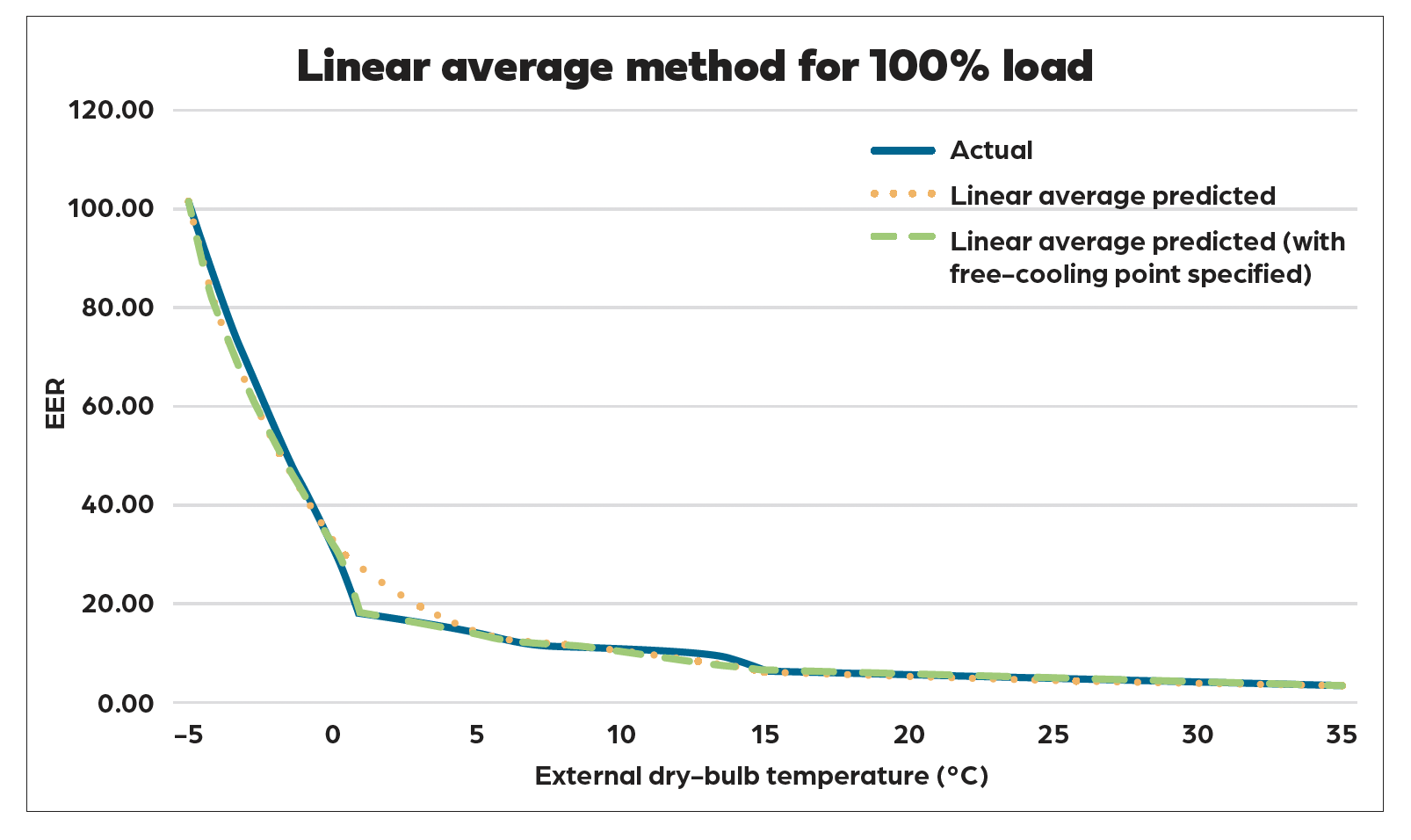
Figure 3: Actual and linear average prediction of EER varying with external temperatures when at 100% load
Applying this methodology for the data provided at all four part-loading conditions (100%, 75%, 50% and 25%) provides a dataset with four EER values at each external temperature. Gaps between these part-loading points can be approximated using a similar approach, to create a complete performance dataset. This set can then be used by engineers to try to perform further complex calculations – such as the application example in Figure 4.
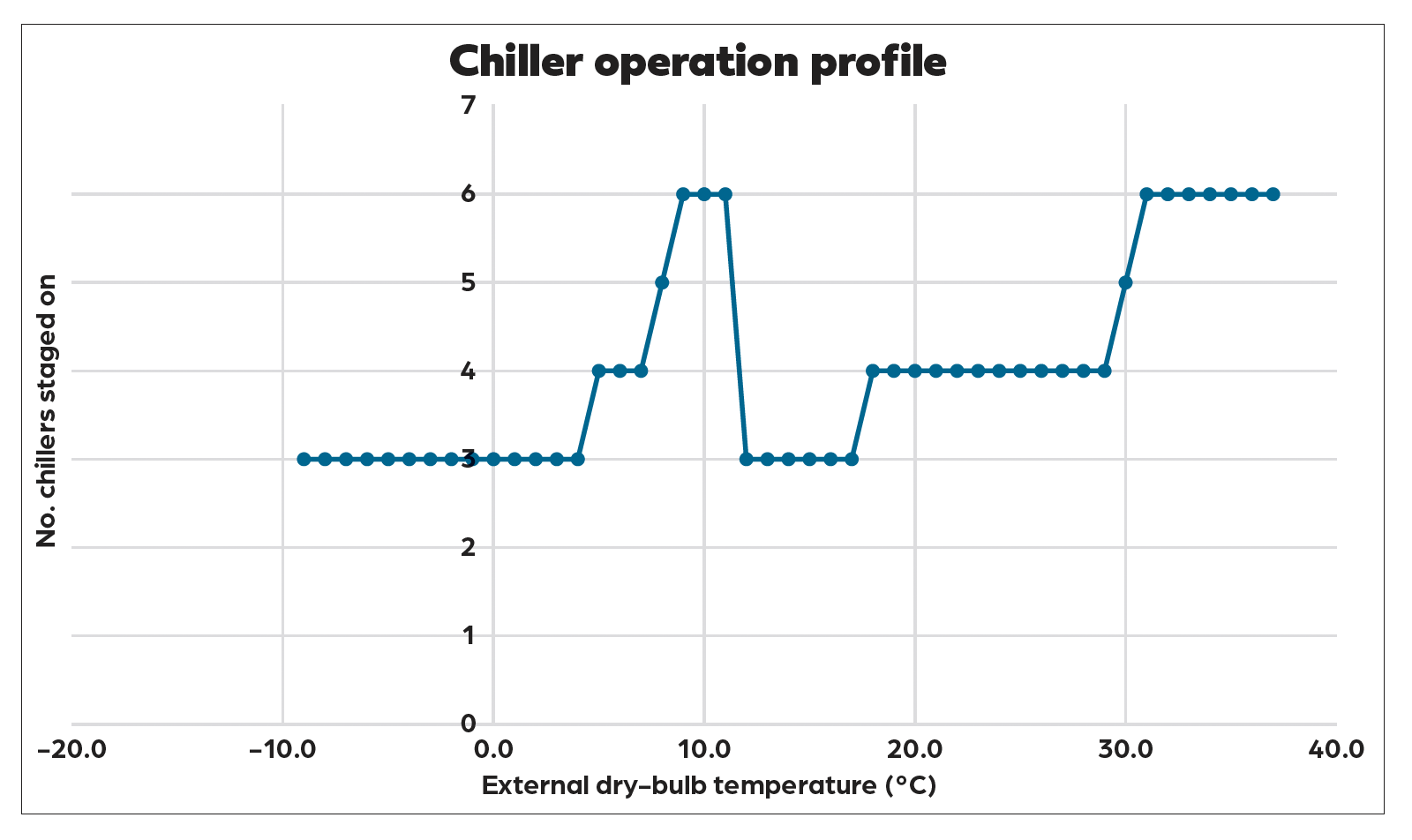
Figure 4: Optimised chiller staging profile
This shows the optimal number of chillers to be used for a given external temperature to minimise annual energy consumption. The profile starts staging the chillers at low temperatures in a conventional manner, only operating the number of chillers that are needed to meet the load – in this example, three machines. However, as temperatures rise, we slowly use more and more chillers, before abruptly returning to the minimum. The reason for this is part-loading, as an individual chiller can stay in full or partial free-cooling mode for longer, delaying the point at which its compressor activates. Overall, this approach will make it more energy efficient to run multiple chillers at part-load, only increasing capacity as the temperatures rise higher. This means running the minimum number of chillers at any time, reducing pumping power.
Whether a control regime such as this could be implemented on site requires further exploration, but the opportunity lies within having a full dataset – so engineers can start having these conversations with manufacturers and thinking more creatively about where additional energy savings could be sought.
The research was presented at last month’s CIBSE IBPSA-England Technical Symposium
About the author
Jakub Borowiec is a mechanical engineer and Peter Owens is associate director at Cundall