The difference between the theoretical and real-world profile of air contaminant levels across a room have been starkly demonstrated by Tom Smith, president and CEO at 3flow.
At the ASHRAE Conference in June, he reported on how models that assume ‘well-mixed’ room air can significantly underestimate levels of room-sourced contaminants at specific locations in the space. He demonstrated that spatial distributions of potentially harmful contaminants, are strongly influenced by ventilation supply and extract locations, geometries, and flowrates.
In his presentation based on his paper Use of an air tracer to investigate air mixing: the truth behind the myth, Smith explained that air quality in occupied buildings was determined by a complex integration of flows of contaminants that might include pathogens and particulate matter from outside, including wildfire smoke.
Activities such as food preparation, off-gassing from finishes, and allergens from flora and fauna add to the cocktail.
Smith noted that concern over a particular contaminant is related to the rate of generation; how much is in a particular space; and how long it remains. This is often referred to as the hazard emission scenario.
This might be explored using the dilution equation: Effective air change rate (ACR’) = Effective volume flow (Q’) / Room volume (V) where Q’ = Q / K with Q being the actual ventilation flowrate and K the ‘mixing factor’ for a space and system.
The mixing factor K makes an allowance for incomplete mixing of the air and is likely to be between 2 and 5, depending on conditions and ventilation system. Lower values of K correspond to good ventilation mixing conditions with a value of 1, indicating contaminants are dispersed uniformly in the space. Under a well-mixed scenario, with a contaminant released in the space, Smith said the ACR is simply Q/V that provides a reduction in concentration with an increase in airflow.
The assumption is that the contaminant disperses into the space until it reaches a homogeneous concentration and then, once the generation stops, it begins to decay. However, the mixing factor does not account for dispersion or spatial variation in concentrations in the space and the decay that occurs after generation stops.
To compare theoretical with actual movement of air, Smith’s team built a hybrid model for the University of California that uses a general dilution equation and other established modelling techniques, including those from the University of California and the US Environmental Protection Agency. The model (available at https://smartlabs.i2sl.org) has input parameters including space dimensions, airflows, and the hazard emission scenario in terms of the contaminant of concern – the model dataset includes 500 possible contaminants.
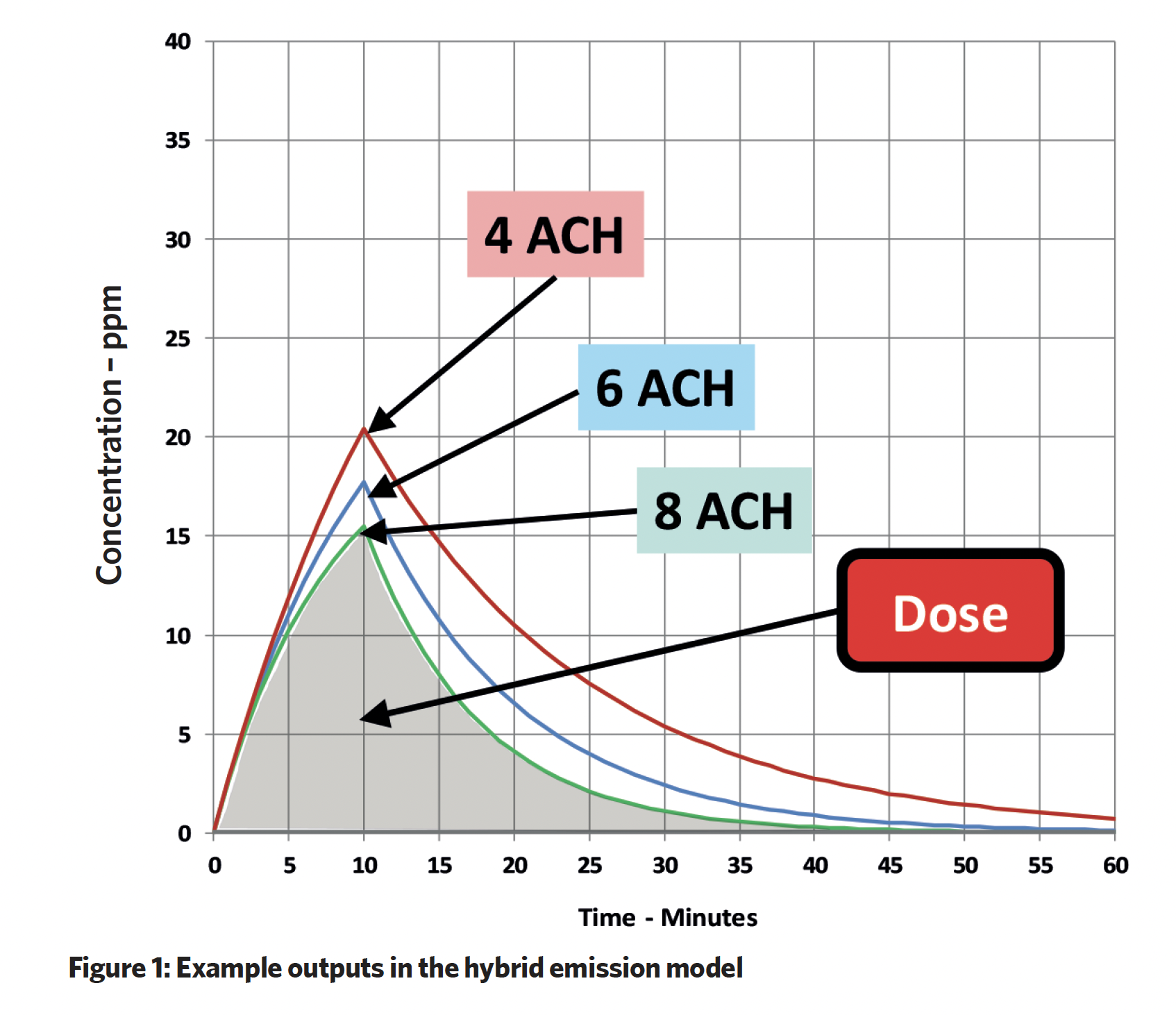
The outputs provide the individual dose, accumulation and decay at different air change rates and the accumulated ‘dose’ area under the curve.
To test how well this model performed compared to the real world, Smith’s team undertook tracer gas tests to test for a ‘well-mixed’ scenario, how uniformly the contaminants disperse and decay and evaluate the results.
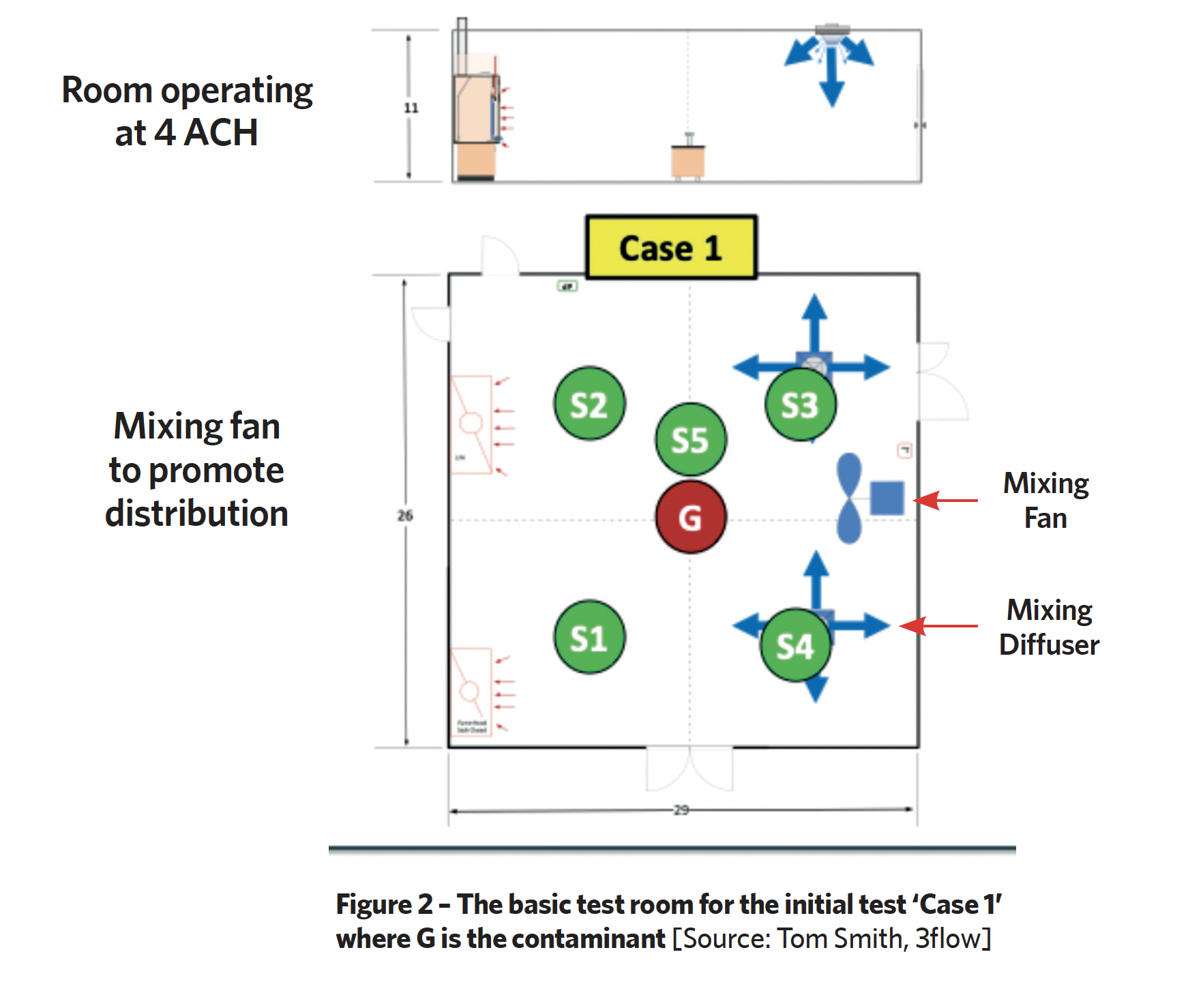
For the initial tests, they employed a 7.62m x 8.8m x 3.05m high test room and added contaminant at the centre, see Figure 2.
In the first test (Case 1), there were two 360-degree supply ‘mixing’ diffusers and two exhaust points at low level. A separate fan was added to mix the air. Using a methodology of 10 minutes of background ventilation, followed by 10 minutes of contaminant generation and 40 minutes of decay, they measured the tracer gas levels across the space and compared it with the model. Sampling points 1 to 5 provided the measured levels of tracer gas; the total doses are shown in the boxes (Table 1).
The spatial distribution concentrations are dispersed and, comparing theoretical and measured data, they are all similar, except for close to the contaminant emission, where there is higher concentration.
To illustrate the effectiveness of the ventilation solution, Smith applied the industrial hygiene concept of ‘effective flow’ VEFF, although he noted that ASHRAE uses the inverse of this, the Ez Factor, to evaluate air distribution effectiveness in a room. The two terms are consistent and enable the calculation of an effective air change rate (ACR). So in Case 1, ACR was 3.4, which compares reasonably to the actual supplied ACR’ of 4.1 (Figure 3 and Table 1).
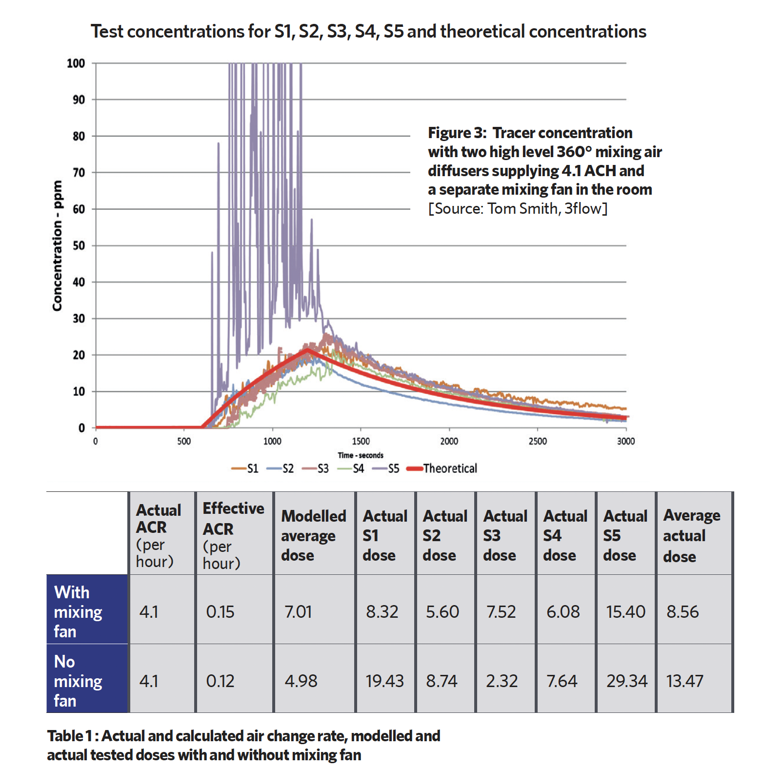
He then removed the mixing fan and, making no other changes, repeated the test to provide results as shown in Table 1.
This indicates a different situation where, although ‘mixing diffusers’ are used, there is no uniformity in mixing and the effective air change rate is 1.5 – just 37% of the supplied air change rate of 4.1. Aside from the near field (S5), the most concerning result was that point S1 received a very high dose.
A training centre used by Smith’s organisation was tested as a real application. The highest dose (of 62 compared with the average of 36) was experienced by those sitting underneath the exhaust point, which also compared unfavourably with the theoretical dose rate of 13. Everyone in the room would have been exposed at a higher level than had been theoretically predicted (that was likely due to stratification).
Smith’s full presentation includes more examples showing startling spatial differences in contaminant concentrations and doses linked to the respective positions, flowrates and geometries of supply and extract points.
View the presentation (at a cost) at bit.ly/CJASHTS23