![]()
Many UK buildings utilise ventilative strategies to comply with the various thermal comfort criteria outlined by building standards. Most ventilation systems employ a fixed position air distribution method that is largely determined by wintertime requirements to ensure good mixing and prevent unwanted higher velocity air movement across occupants.
This approach limits the impact that increased airflow during summer periods can have on improving perceived thermal comfort from occupants as a result of convective heat transfer. To illustrate the application of CFD, this article will focus on how CFD has been employed to examine the room air movement created through a high-level, fan-assisted outdoor-air ventilator, to determine if summer thermal comfort may be improved despite ambient temperatures being high.
The example CFD exercise will compare the thermal comfort experienced by classroom occupants in a typical summer condition for two electrically controlled modulating grille outlet blade positions, upward and downward, as shown in Figure 1. In the blade ‘up’ position, airflow is directed 20 degrees upwards, towards the ceiling. This arrangement optimises thermal comfort during winter conditions, minimising airflow across occupants.
In the blade ‘down’ position, the airflow leaves the grille at 20 degrees downwards, towards the occupied zone. Here, the airflow is moved directly over the occupants, and this will provide the subject for the CFD investigation in this article.
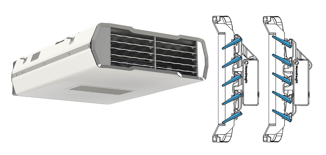
Figure 1: Upward and downward outlet motorised blade positions (Source: Monodraught)
The opportunity to apply CFD tools is becoming increasingly available as the interfaces become more intuitive for the CFD non-specialist. Increasing numbers of CFD code developers offer web-based, or application specific, interfaces to their packages as software as a service (SaaS) solutions that are ‘cloud-based’.
This provides a great opportunity for the building services engineer to try out applications of CFD, as several vendors provide free or low-cost entry-level access. For cloud-based implementations, there is no requirement for hardware or software installation or maintenance investment, aside from a standard laptop computer or tablet.
However, the underlying principles are complex, and every CFD simulation is, as the name suggests, an approximation of the real world.
The methods employed and the granularity of the digital interpretation of the physical application will impact significantly on the reliability of the result.
Velocity, pressure, temperature, density, and viscosity are the main properties that are considered simultaneously when conducting an examination of fluid dynamics. The physical phenomena, such as turbulence and mass transport of air, will vary enormously and are categorised into kinematic, transport, thermodynamic, and other miscellaneous properties.1
The Navier-Stokes equations are commonly applied to examine changes in these properties during mass flow and/or thermal interactions, and are applied in investigations that include a diverse range of applications, including: weather prediction; car design; pollution and flood control; the study of climate change, blood flow, ocean currents, tides, turbulence and shock waves; the representation of water in video games or animations;2 and, of course, building services engineering.
The set of equations is based on the principles of conservation of mass, momentum, and energy that are often solved for many thousands or millions of individual elements, or cells, that have been defined by the mesh (as discussed below) that represents the volume of the room, the content, and its boundaries.
The conservation of mass is expressed in terms of the continuity equation, where the rate at which the mass enters a system is equal to the rate at which mass leaves the system plus any accumulation of mass within the system. Conservation of momentum is described by Newton’s second law, such that the sum of all the forces on the element must equal the mass of the element times its acceleration.
This might cause the element to speed up, slow down, or change direction, depending on the direction of the force and the directions in which the object and reference frame are moving relative to each other.3 And, finally, the conservation of energy is an application of the first law of thermodynamics, that energy cannot be created or destroyed but is just transformed from one form into another.
The non-linearity of the governing equations means that fluids are inherently chaotic, and therefore highly sensitive to changes in initial or boundary conditions (such as the angle of the outlet blade). This means that a change in any input variable can produce a vastly different response to a seemingly small perturbation in the input variable.
This non-linearity, along with the complexity of the physical geometries, means that an accurate analytical solution (such as directly employing the Navier-Stokes equations) is often not possible, and so numerical methods are used to iterate solutions within a ‘discretised’ domain until the simulation closely approximates the analytical solution.
The numerical solution of the differential equations cannot produce a continuous distribution of the variables over the whole solution domain (such as the room volume) at a single pass, so the aim is to produce a set of discrete values at many thousands (or millions) of nodes (each one surrounded by its small volume) that cover the solution domain.4
Properties
k – kinetic energy
ω – often referred to as the turbulent frequency, the rate at which turbulence kinetic energy is converted into thermal internal energy per unit volume and time6
ε – specific dissipation rate at which velocity fluctuations dissipate7
This is the basis of the finite volume method that is commonly employed to handle this kind of problem. The strategy works by the ‘meshing’ of continuous geometries into grids of discrete, interconnected volumes known as cells. Most methods employ algorithms based on the Reynolds-averaged Navier-Stokes (RANS) equations.
RANS turbulence models were derived by time-averaging the Navier-Stokes equations – this makes the process less complex to model numerically than considering every minute deviation from the average at a particular point, as the fluid properties vary chaotically in the turbulent air stream.
These are then applied to iteratively evaluate fluid parameters (such as velocity, pressure and temperature) for each of these cells, until a converged solution is met. The finite volume method is a particularly popular choice for CFD, as it rigorously enforces conservation, and is flexible in terms of both geometry and the variety of fluid. It does not limit cell shape and mass, momentum or energy is conserved even on coarse grids.
There are several efficient, iterative well developed ‘solvers’.4 CFD solvers transform the defining momentum and thermodynamic laws into algebraical equations, and can efficiently solve these equations numerically.
Commonly employed solvers for incompressible, steady-state flow regimes include the two-equation shear-stress transport k-omega (SST k-ω) eddy-viscosity model to provide an approximation of RANS equations (see ‘Properties’ boxout for descriptions).
The use of a k-ω formulation in the inner parts of the boundary layer makes the model directly usable all the way down to the wall through the viscous sub-layer. The SST formulation switches to a k-epsilon (k-ε) behaviour in the free-stream, and thereby avoids the common k-ω problem that the model is too sensitive to the inlet stream turbulence properties.
The SST k-ω model is by no means perfect but is likely to be more effective than employing a single k-ε model.5
Creating a high-quality mesh to represent the domain is a critical factor in ensuring CFD simulation accuracy. A fine mesh with a grid of small – possibly irregularly-shaped – interconnected cells will typically yield a higher-quality mesh, but the computational cost will be significantly increased.
A lower-quality mesh (which might also be a coarse mesh) will not only result in inaccurate simulation results, but may also cause ‘convergence’ difficulties. (Convergence is a measure of how the iterations are converging towards an acceptable resolution of solution.)
Where a quick solution is needed – for example, at concept design stage – it may be acceptable to employ a less-refined mesh to reduce set-up time. However, most analyses will require some time and effort to set up the mesh using the different methods and controls made available in the software.
It is normal to start with a coarse mesh and then gradually refine the mesh for specific areas of interest. Fortunately, the speed of solution in simple models – particularly cloud-based systems – provide ready opportunities to experiment.
To ease the process, most CFD packages include automated mesh generation tools (both static and dynamic) that, if set up correctly with good-quality definitions of boundaries – such as the walls and the grille outlet blades – and volume fluid properties, are likely to be adequate for most general building services investigations. While a mesh may contain millions of nodes, that fact alone does not necessarily equate to quality.8
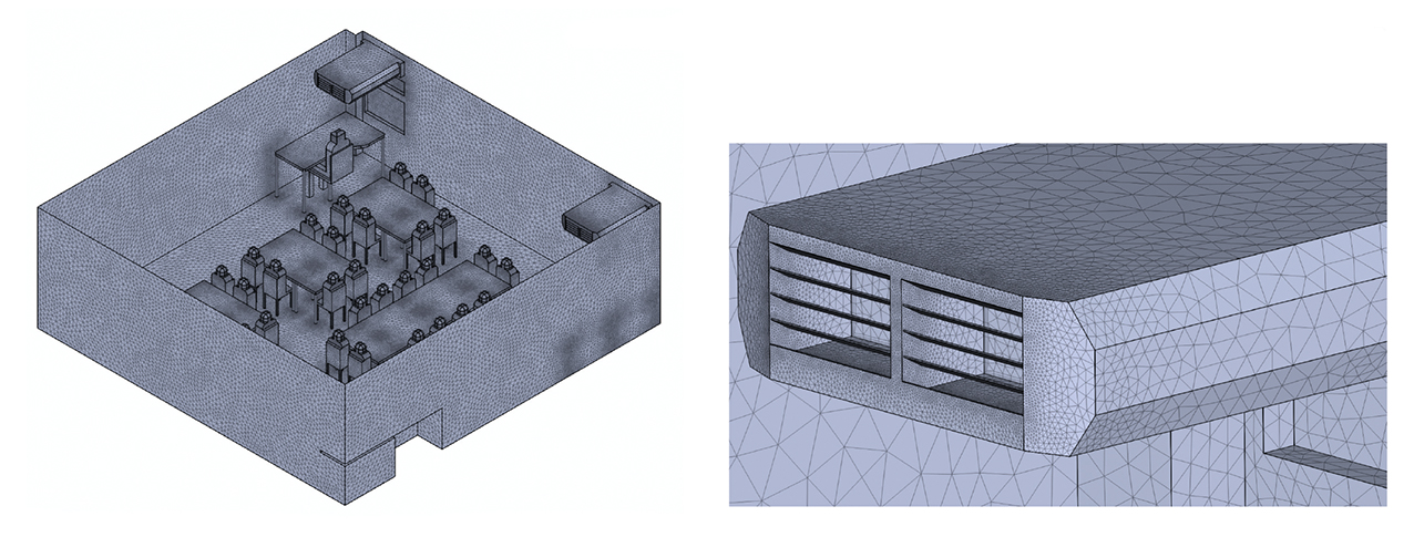
Figure 2: The surface mesh structure of the ‘blade up’ fluid domain. Both domains contained approximately 12 million cells (Source: Monodraught)
Having set up the geometry – which can normally be imported from CAD or created directly within the CFD package – and defined the boundaries, volumes and initialised conditions, the mesh will be generated and the pre-processing stage is complete.
During the processing stage, after each iteration, at each cell, a new value for a variable is determined from VariableNEW = VariableOLD + α (VariablePREDICTED – VariableOLD) where α is the relaxation factor.
An α <1 (under-relaxation) will slow down the convergence rate but increase the stability, and as α moves above 1 (over-relaxation), it can sometimes accelerate the convergence rate but will decrease stability.
The difference between the previous result and the current result, the ‘error’, is known as the residual. As these errors decrease, the results are reaching values that are changing less and less with each iteration and so the solutions are converging. If these errors increase, the solution is said to be diverging. The generally accepted starting point is to employ the software default values of relaxation factors.
Example
Four CFD simulations were used to model the steady state airflow characteristics in the example classroom, and to use the output to provide thermal comfort profiles, expressed in terms of predicted mean vote (PMV) for the two grille-blade positions – up and down – and for two different external air temperatures – 26°C and 29°C.
Under-relaxation factors were also adjusted for convergence, with the analysis stopping when global residual values for continuity, energy and turbulence were evaluated below 10-5. The airflow supplied by each unit was 130L.s-1 and 180 L.s-1 (respectively, for the different external air temperatures) with two units fitted to each room, to emulate the typical response of an installed unit’s control strategy.
The geometry of the room was created in CAD, and simplified block geometries were used to represent the occupants and ventilation units. The internal components of the ventilation systems were not modelled, and a simple boundary condition stating a flow velocity and temperature was used, to reduce computational time.
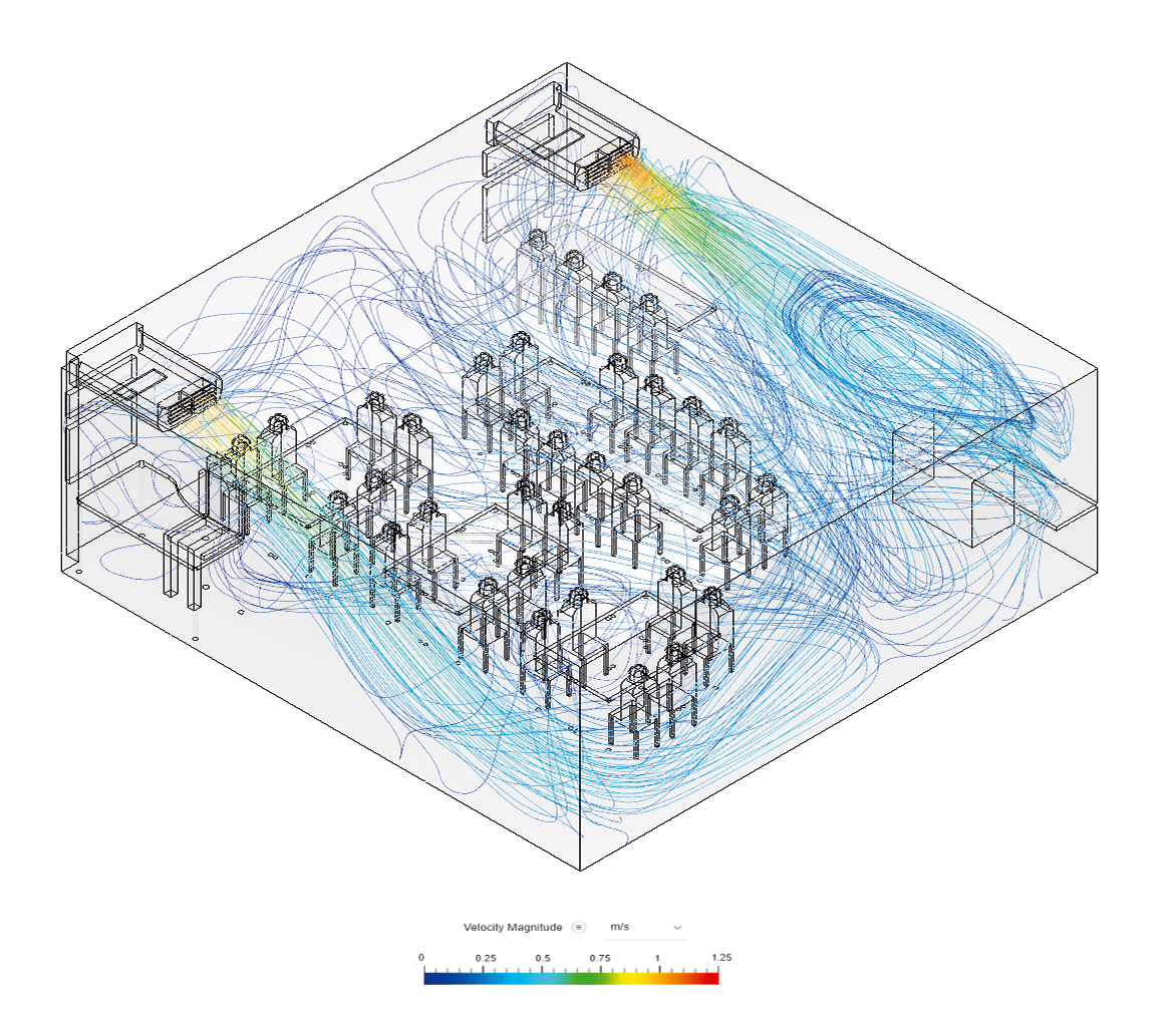
Figure 3: Example visualised output of steady-state velocity streamlines when the blades are facing down, with each unit supplying 130L.s-1 with air supplied at 26°C (Source: Monodraught)
The CFD automated mesh algorithm was employed, having been set to form five automatic prism layers within a close proximity to any boundary within the domain, as a means of capturing fluid-solid interaction in detail (see examples in Figure 2).
In the post-processing phase, the simulation output was used to provide data for both PMV calculations and visual interpretations, such as the velocities shown in Figure 3. This indicated that, under the modelled conditions, both blade positions are predicted to provide suitable velocity, temperature, and thermal comfort profiles to meet the criteria set out within BB101.9 (The results of the analysis were also successfully evaluated against the CIBSE, ASHRAE and BS EN ISO-773010 design criteria.)
The output indicated that the distribution of incoming airflow within the room would be even, and throws should cover the width and depth of the room. Thermal comfort was indicated as remaining between a PMV of -0.5 and +0.5 within the occupied zone at a height up to 1.4m.
Compared with the ‘upward’ position, the ‘down’ position for the blades improved the PMV score by 34% for the ‘normal’ summertime analysis with an external temperature of 26°C, and improved it by 28% for the ‘adverse’ summer analysis when the external temperature was 29°C.
This article provides a small fraction of the depth and complexity that CFD analysis requires, and the solutions that it offers. To create meaningful and reliable output requires the user to develop expertise, or to utilise the services of a professional who specialises in the field of CFD for building services engineering.
© Tim Dwyer, 2021.
■ With appreciation for the technical input by Dr Esfand Burman of IEDE, UCL.