![]()
No matter the skill of the designer, a commercial building’s circulating heating or cooling water system, particularly if it includes constant-volume elements, is unlikely to be self-balancing. This CPD will explore the proportional balancing method as a means of setting such systems for effective operation.
Pipework systems, such as those used in cooling and heating systems in buildings, will not operate as intended without proper commissioning. Inadequate balancing of constant-volume systems will lead to poor control of terminals such as fan coils, heating and cooling coils, radiators, convectors and panels.
It is likely that in variable flow systems and, increasingly, systems that employ PICVs, there is limited need for balancing devices. However, for many legacy systems that have been modified or simply need recommissioning, larger systems, and constant volume systems, it is important that appropriate devices are included for regulating and measuring the flowrates in the piping circuits to allow onsite balancing. For all systems, the decisions on commissioning need to be taken at the design stage and well before work commences on site.
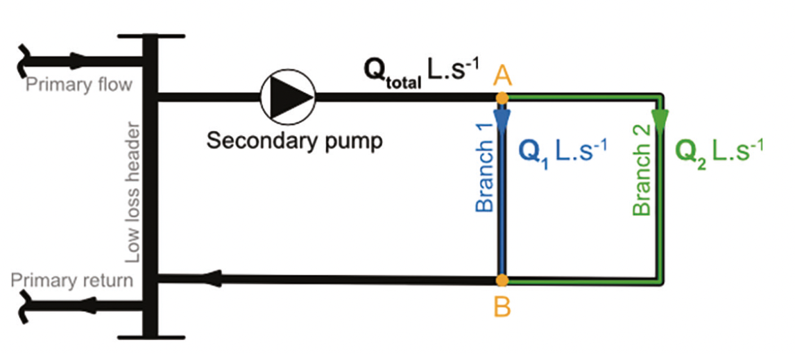
Figure 1: Simplified two-branch pipe network
Although many contemporary commercial installations are designed as variable volume systems, potentially they still include sub-systems that have constant-volume requirements. Also, where PICVs control a sub-network that serves more than one terminal unit (for example, multiple fan coils), there may be the need to balance these terminal units against each other.
For those terminals (hydraulically) furthest from the pump, lack of balance could mean an inadequate flow of water, and those closer to the pump may suffer from poor control as their control valve struggles to overcome a high-pressure differential (which results in a low valve authority). Poorly performing terminals can encourage users and building occupants to ‘tweak’ the system, which, in turn, is likely to exacerbate poor environmental control, increase unnecessary energy use and lead to poor occupant comfort and productivity.
As discussed by Roger Legg1 – and as recommended by BSRIA2 and CIBSE3 – a standard, methodical way to balance pipework systems is known as proportional balancing. This employs the simplified relationship for fully developed turbulent fluid flow, Δp = RQ2, where Δp = pressure drop, kPa, in a particular pipework section, Q = volume flowrate, L.s-1, and R is a constant of proportionality that reflects the resistance to flow in the particular pipe network from pipe friction, turbulence and losses through fittings and components.
A simplified representation of a network with two branches, with no valves or heat exchange devices shown (for clarity), is illustrated in Figure 1.
Branches 1 and 2 have volume flowrates Q1 and Q2 and resistances to water flow R1 and R2. The pressure drop between A and B is the same for both branches and so Δp1 = Δp2 = R1Q12 = R2Q22. So, the ratio of the flows Q1⁄Q2 = 
and this will remain a constant so long as there is no change in the resistance in either branch. With no (possibly further) valve adjustment, the ratio of the flowrates will remain the same irrespective of any change in the total flowrate, Qtotal. Practically, this will mean that once the ratio Q1⁄Q2 is set to match the ratio of the required design flowrates, the flows in those two branches will remain at that ratio. (Typically, this ratio would be obtained by closing a regulating valve.)
This is the basis of proportional balancing – methodically setting up pairs of sub-networks to a desired flow ratio. As each, increasingly larger, sub-network is added to the tree of balanced sub-networks, it is set to be in proportional balance with the previously balanced sub-networks.
Subsequently, when the total flowrate is adjusted to provide the design total flowrate – by, for example, reducing the pump speed – the relative balance of the flowrates will be maintained, and all branches will receive their design flowrates. (An example balancing process is provided later in this article.)
In the very simple circuit of Figure 1, it may be reasonable to guess that, if the pipe sizes are the same, R2 is greater than R1 (owing to the extra pipe length) and that, before any balancing, the flow through branch 2 will be least favoured.
However, that is not a certainty, as the fittings – such as the bends and tees – and components – for example, control valves and heat exchangers – and the quality of the installation, which can have a significant impact on resistance, may not be fully apparent until the pipe network is installed on site and subsequent measurements are taken.
The flowrate through any fixed resistance element is usefully characterised by Q=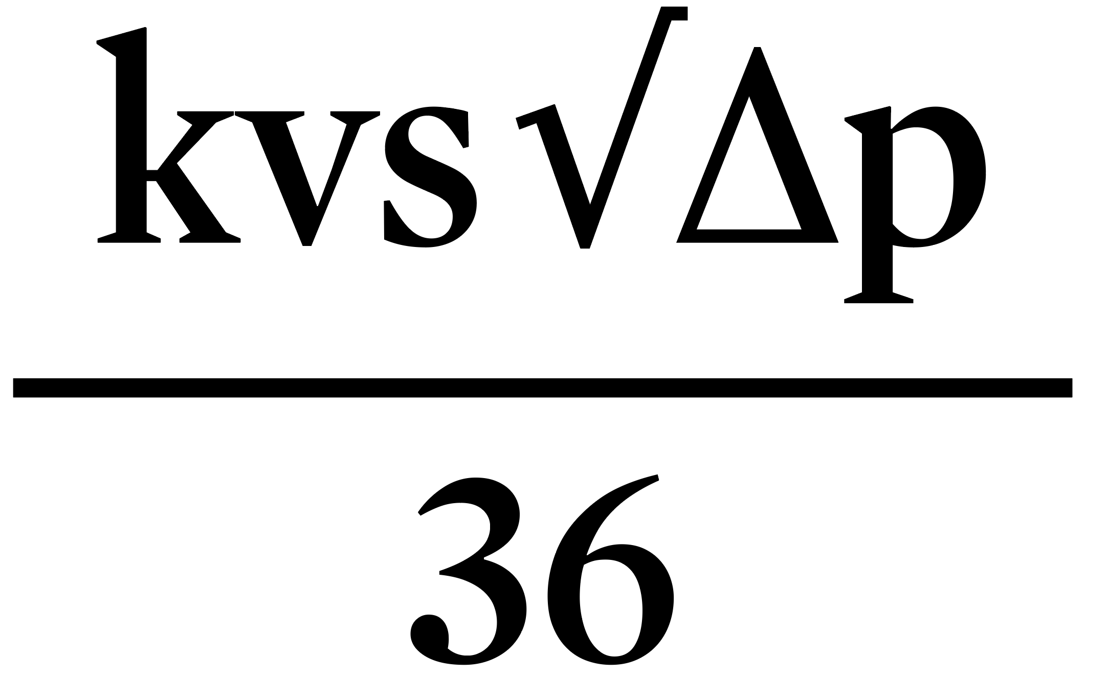
where Q = volume flowrate, L.s-1, Δp = pressure drop across the element, kPa, and kvs is the flow coefficient for the fixed resistance.
Orifice plates (OPs) – and, more rarely, venturis – can be employed as flow-measuring devices (or ‘metering stations’). OPs may be close-coupled to a commissioning valve, or separate items (such as shown in Figure 2). The flowrate coefficient, kvs, for the measuring device will normally be supplied by the manufacturer. Self-sealing pressure tappings allow a manometer (see panel, ‘Measuring the flow – digital manometers’) to be connected to the flow-measuring device, which are normally suitable for cold and low-temperature hot water (LTHW) systems.
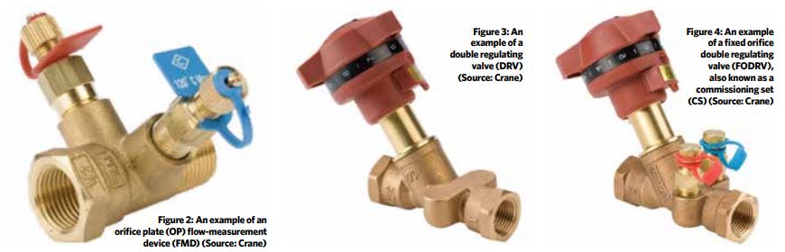
Commissioning valves are used to add resistance to circuits to balance the system, and are usually placed in the return pipework from the load(s). Most commonly in commercial systems, this will be a double regulating valve (DRV) or a commissioning set (CS).
A DRV is used for regulation and isolation, and is often an oblique pattern globe valve (Figure 3). Once a branch has been regulated (for example, brought into proportional balance), the valve can be ‘locked’ at this setting. Then, if the valve is subsequently closed to isolate the circuit, when reopened it cannot be mistakenly opened beyond its original setting.
DRVs typically include a scale on the handwheel or valve stem to provide a visual record of the valve setting. The DRV may be close-coupled, or integrated with an orifice plate to form a fixed orifice double regulating valve (FODRV), and is sometimes referred to as a commissioning set (CS), as shown in Figure 4.
The pressure difference measured between the two points on the CS, at a particular opening position, may be converted to a flowrate through a specific flowrate equation for the device or by using the flow chart for the valve.
Before commencing the commissioning process, the installation must have been installed in accordance with the specification; flushed and cleaned; successfully pressure tested; and filled, treated and vented. The whole system should be in a safe and operable condition, and all the commissioning valves should be fully open and control valves set to allow full flow through the terminal units. This method will not be appropriate to systems that have been designed with reverse-return pipework.
The pump must first be tested to confirm that it is able to provide sufficient water power to satisfy the demands of the designed system. If the pump had been undersized, it would be impossible to achieve design flowrates and much time could be wasted in futile attempts to commission the system.
A ‘closed head’ test is undertaken by operating the pump and then gradually closing the pump outlet isolation valve, and noting the pressure differential measured across the pump when it is closed. This can then be checked against pump curve from the manufacturer’s details, and a parallel, corrected, pump curve (based on the closed head test) can be sketched if the closed head pressure differs from the manufacturer’s details.
The outlet valve is then gradually opened and the pressure differential at full flow is plotted on the (potentially corrected) curve. The required design flowrate is also plotted on the curve to confirm that it is practically attainable with the pump and, if not, some further investigation will be required.
Measuring the flow – digital manometers

Figure 5: Digital manometer kit (Source: Crane)
Properly calibrated digital manometers, connected by tubing to measuring stations, are typically employed when commissioning systems. Modern variants (such as the example in Figure 5) are available to measure pressure differences up to 600kPa and, because of their ease of application, have practically replaced the previous generation of liquid manometers (the so called ‘water box’).
Such manometers are able to employ the characteristics of commissioning valves (using the flow coefficient for the device, kvs) that can be pre-programmed in the electronic firmware to provide a direct reading of the water flowrate. The connecting tubes incorporate self-sealing connectors; these may be push-on units for quick connect/disconnect, but more usually a threaded fitting is used with a cap to protect the connection from dust.
It is not necessary to balance flowrates within a group of loads precisely. Allowable tolerances of balance are given in CIBSE Commissioning Code W3.3 Notably, a closer tolerance is required when the heating system temperature difference (ΔT) is greater than 11K.
The pump initially should be set so that it is delivering approximately 110% of the design flowrate. As noted in CIBSE Code W ‘it may be necessary to vary the pump speed (if the pump is a variable speed pump) or close valves elsewhere in the system’. Even with this margin, it still may be necessary to open the main balancing valve (valve K, if it had been previously partly closed) or increase the pump speed (or potentially, increase impeller size) when the balancing is finished to bring the water flow to design conditions.
With all regulating valves (and control valves) still fully open, the flowrate is measured through each of the branches. The ratio of 
is used to determine percentage design flowrate (%DFR). The branch (hydraulically) furthest from the pump will have the lowest %DFR (although it may not be physically the most distant) and so be the index circuit.
If all the branches are of the same configuration, the most distant should be the index run (in this case Floor 4) – if not, it indicates that there may be some blockage, or a control valve is not fully open to the load. To progress through the method of proportional balance, one of the last two (parallel) branches must be the index circuit. If this is not the case, then an initial resistance adjustment will be needed to make it so (for example, by partly closing a commissioning valve).
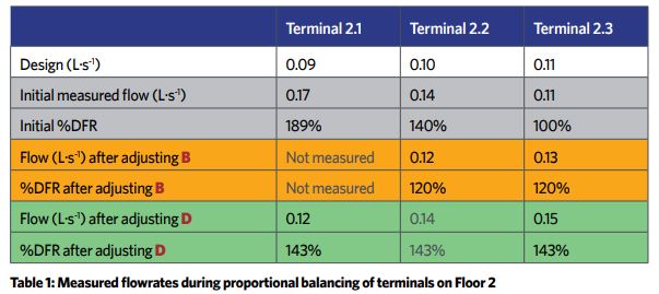
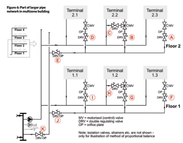
As an example, consider the proportional balancing of the three terminals on Floor 2, with the steps indicated in Table 1. In this case, the initial measurement confirms the index as Terminal 2.3 (that is, it is the least favoured).
Valve A is left fully open and B is adjusted to obtain the same %DFR for T2.3 as for T2.2. This would employ two manometers, one connected to the index OP and one to the OP in the branch being adjusted (in this case B). T2.2 as for T2.3 are now in balance and valve B should have this maximum opening ‘locked’.
The same process is undertaken for T2.1 by adjusting valve D and comparing the flows through OP A and OP D until the %DFRs are the same. All three terminals are now in balance, and although all have a %DFR of 143%, any flowrate changes in the system will affect flowrates through these units equally.
Each of the bypass DRVs can then be adjusted in turn (that is, C and H). The control valve is closed to load and open to bypass, and then the respective OP is used to measure the flow through the fully open bypass. The bypass DRV is adjusted (and locked) so it has the same flow as has already been measured through the associated load (in the previous step).
The same process (which would have commenced on Floor 4) is completed across each of the floors and then the four floors are proportionally balanced with each other using the branch commissioning sets (that is, E and J plus those on Floors 3 and 4). Once the whole system is in proportional balance, the total flow can be regulated down to the design flowrate by adjusting the pump speed or, alternatively, using regulating valve K.
A permanent record of the balancing process should be maintained – BSRIA BG2-2010 includes example sheets that may be used.
© Tim Dwyer, 2021.
Further reading:
See CIBSE Commissioning Code W and BSRIA BG2-2010 for more extensive applications and detail for commissioning water systems.
References:
- Legg, R C, Air conditioning system design, Chapter 16, Butterworth-Heinemann, 2017.
- BSRIA BG2-2010 Commissioning water systems, BSRIA 2010.
- CIBSE Commissioning Code W: 2010 Water distribution systems, CIBSE 2010.