Variable air volume (VAV) is well established in the global air conditioning market, having been embraced in the US more than half a century ago. This preceded the 1970s energy crises (that subsequently heightened the interest in VAV) but, as noted by Shepherd in his seminal work,1 it was quickly adopted as ‘enlightened engineers and building clients appreciated the potential of VAV techniques’.
In building services engineering, when considering flow of air through ducts, the pressures are such that the air is considered as being ‘incompressible’ – the volume does not change with pressure (although the specific volume will alter as the air temperature varies).
As air flows along a duct, it is convenient to consider it in terms of static pressure, pS (Pa), velocity pressure, pV (Pa), and total pressure, pT (Pa) where
pT = pS + pV, and where velocity pressure, pV = 0.5 x fluid density x (air velocity)2 = 0.5 ρ c2, as shown in Figure 1.
Considering the flow of air through a duct (as in Figure 1), the volume flow, q (m3.s-1), may be determined from the average velocity of the air, c, multiplied by the duct area, A (m2). Typically for air systems, a density, ρ, of 1.2kg.m-3 is used (this varies +/- 4% across the range of typical HVAC conditions) so pV is commonly noted as being 0.6c2. (In a ducted air system, the velocity pressure of the air may be determined using a pitot-static tube traverse or, more practically, in an operating system through a fixed measuring device such as velocity tubes or a pitot grid.)
As explained fully in CIBSE Guide C1, the ‘Darcy equation’ is used to provide a relationship between the parameters of a conduit (such as a pipe or duct) and the pressure drop (because of frictional resistance) in the fluid (water or air) flowing in that conduit:
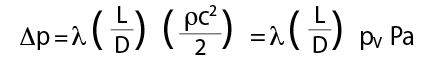
where λ = friction factor; L = length of conduit (m); D = hydraulic diameter (= 4 x area/perimeter) of conduit (m); c = velocity of fluid (m.s-1); ρ = fluid density (kg.m-3); and p = pressure (Pa).
Reynolds number, Re, is applied to determine the friction factor, λ. The Reynolds number – Re = ρ c d/μ, where μ is the dynamic viscosity of the fluid (Pa.s) – characterises the flow regime of air in a duct. Air viscosity does not alter significantly across the range of typical conditions in HVAC ductwork, and the viscosity for air at 25°C, 0.18 × 10⁻⁴Pa.s is commonly used as a representative value.
Flow is considered as laminar (streamlined) when Re < 2,300 and turbulent when Re > 3,000. When flow is laminar, the friction factor is given by the Poisseuille equation, λ = 64/Re. However, the velocities in HVAC ductwork will inevitably produce turbulent flow. When turbulent, the friction factor will be influenced both by variations in Re (that in a particular duct is proportional to the velocity) and, to a lesser extent, the ‘relative roughness’ – – where k is the surface roughness of the duct (for example, for new galvanised steel, k = 0.15mm) and D is the hydraulic duct diameter (measured in a unit consistent to that of k). The relative roughness will only alter for a particular duct as the surface characteristics change – for example, as the duct ages or becomes contaminated.
For turbulent flow, the implicit Colebrook-White equation, or one of the many explicit alternative equations such as the Haaland equation (as used below), is applied to determine the friction factor where
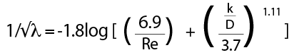
It is generally considered that the friction factor alters only slightly for a particular duct system, as the flowrate varies through the duct within a range of typical air velocities. (In reality, this may be an oversimplification as, at lower velocities – of approximately < 5m.s-1 – as volume flowrates and velocities vary, the effect of the change in Re will significantly alter the friction factor.)
Assuming a constant friction factor, as the air velocity (and hence volume flow, q) changes – and assuming all other parameters in the Darcy equation are constant – the duct pressure drop is proportional to the square of the fluid velocity, and to the square of the volume flowrate, ∆p ∝ q2. This applies to the whole duct flow system including fittings as long as the geometry stays constant (for example, damper settings remain unaltered).
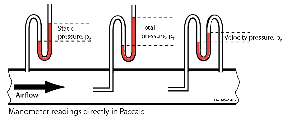
Figure 1: The pressures in a duct with flowing air
Since ∆p ∝ q2, then for any particular flowrate ∆p1= R q12, where R is the characteristic resistance of the ducted system, R may be established from the design pressure drop and flowrate and can be applied to discover the system pressure drop at other air flowrates.
The power, P (W), required to move the air through a ducted air system with a total pressure drop of ∆pT may be determined from P = q ∆pT and since ∆p ∝ q2, significant savings are achievable as the required air power (and so, fan power) will reduce by the cube of any reduction in volume flow.
This is the key driver for the application of multizone VAV systems in buildings that have multiple zone loads that peak at different times of the day. In a constant air volume multizone system (CAV), the cumulative total of the peak airflows to supply the zonal design (peak) loads must be supplied continuously, whereas VAV needs to supply air only to meet the concurrent zone loads that, as shown in Figure 2, offer the potential for significant fan energy savings.
Early VAV installations – which revolutionised the air conditioning marketplace of the 1960s – were controlled using, in today’s terms, relatively basic pneumatic or electrical controllers, but they were still able to provide systems that delivered a step change in reducing energy consumption compared with constant volume multizone air conditioning. The prevalent pneumatic controls were effective in controlling zone temperatures and system static pressure, but provided little or no ‘data’ that could be used by the operator or for overall systems management. The mechanical control techniques of the time that were used for varying the volume flow delivered by fans similarly lacked the connectivity, flexibility and performance of today’s digitally controlled variable speed motors.
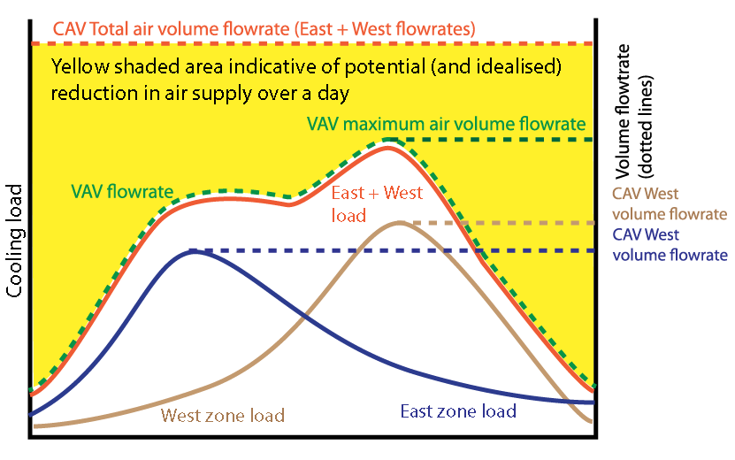
Figure 2: Idealised and simplified representation of reduction in air supply volume over a day for two zones with VAV compared to VAV
There are many variants of VAV systems. The simple VAV system, shown in Figure 3, provides the characteristic elements where each of the terminal units receives primary air from the central air handling unit (AHU) at the same temperature. The flow through the supply fan is typically modulated to maintain the supply air static pressure so that it is sufficient to supply the required air though every terminal, while attempting to keep duct static pressure as low as possible. The exhaust fan flow will be varied to meet the needs of building pressurisation and the supply air flowrate.
The central plant is able to use an economiser cycle (mixed air), but controlled so that zones supplying minimum airflow are still providing an appropriate proportion of outdoor air. Traditionally, the primary supply has been at a fixed temperature and is often at about 13°C, since the original role of the VAV system was to provide only cooling to core areas in buildings. Some systems have evolved to include seasonal (or continuous) reset in the supply air temperature so as to meet space load requirements more effectively (for all zones) while maintaining outdoor air requirements and optimum distribution costs.
The terminal unit (such as the schematic example in Figure 4) contains a butterfly damper, which modulates so the flow of cool air into the conditioned space is sufficient to offset the cooling load in the space. VAV terminal units often integrate reheaters to meet local heating loads to, for example, offset perimeter winter heat losses. As described more fully in CIBSE Guide H (section 5.8), the air supply is typically controlled from the space temperature with a cascade (or reset) controller. This offers temperature control and damper operation to regulate airflow, using an integrated pressure sensor for the airflow measurement.
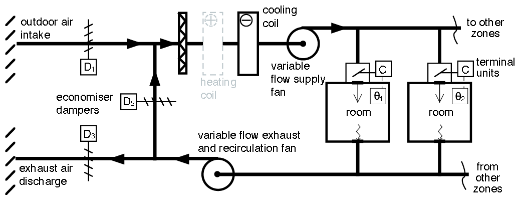
Figure 3: A simplified basic VAV system
The significant advantages delivered by VAV systems – including the reduction in fan power and reheat compared to a CAV – are not without challenges, such as the lack of zonal humidity control; ensuring sufficient outdoor air supply to individual zones; and delivering appropriate room air movement at maximum terminal turn-down. Typically, VAV boxes have been selected to be able to turn-down to 30% of maximum flowrate to maintain air distribution. At lower flowrates, cold air ‘dumping’ and the lack of mixing when supplying reheated air have often been associated with a poorly conceived or operated VAV system.
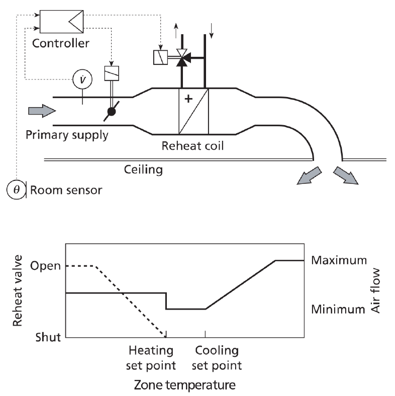
Figure 4: A generic pressure-independent VAV terminal unit. It is ‘pressure-independent’ because the room sensor directly influences the volume flow of the primary air through the employment of two cascading control loops: the first sets zone supply temperature and the output from this resets the airflow required; and the second controller varies damper position to maintain flowrate independent of the primary air pressure. The flowrate in this example for the heating is set above the minimum (for cooling) to meet the maximum heating load (at an appropriate maximum supply temperature) while ensuring reasonable air distribution (Source: CIBSE Guide H, 2009)
There have been many adaptations of simple VAV to overcome some of these deficiencies. For example, where there is a high diversity in a zone load – for example, in meeting rooms – fan-assisted terminals (that recirculate and mix room air with the primary air supply) have been employed to allow a constant air volume to the zone, so ensuring an appropriate air distribution and ventilation efficiency while the primary supply air to the zone box is varied. This can additionally be combined with reheat that is activated when both the primary air has been reduced to a minimum and the heat recovery from the recirculated room air is insufficient to maintain required room temperature. Variable geometry diffusers – such as the concept in Figure 5 – have been developed to maintain supply velocities at lower flowrates that are sufficient to maintain the Coand effect across soffits to maintain the desired air distribution.
The advent of digital controls and efficient variable-speed motors has spawned a multitude of systems that are able to efficiently maintain good quality room conditions.
For example, as reported by Taylor,2 digital signal processing can work to deliver stable supply flowrates that are significantly lower than those normally specified by the manufacturer. Such controllability may be employed for ‘time average ventilation’ that varies the volume flow over a period of time (for example, 15 minutes) averaging below the normal minimum flow that benefits from the capacitive qualities of the room air volume – mass, thermal and contaminant – to maintain an acceptable, time-averaged, internal environment.
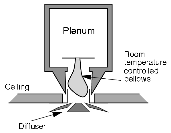
Figure 5: Concept variable-geometry VAV diffuser
Similarly controlled ‘purge cycles’ can be employed to reduce zone ventilation during unoccupied periods by boosting the rate of airflow immediately prior to occupation.The possibilities and complexities in the control and monitoring of multizone VAV make commissioning and troubleshooting increasingly complicated. However, as proposed and explained by Brambley,3 software modules for fault detection, isolation and correction for VAV terminal boxes that work in conjunction with building management systems can be deployed, which will automatically identify, signal and seek to resolve faults.
One of the significant recent shifts in VAV is its increased adoption as a solution for small-scale single-zone air-conditioning applications such as cafés, restaurants, teaching spaces, offices and shops. The zone sensor is used to vary both the cooling or heating capacity and the fan speed. These compact package units include efficient variable speed fans and use contemporary optimised subsystems such as direct expansion (DX) split cooling with variable speed compressors, fan-coil units, heat pumps and high-efficiency particulate filtering. Increasingly, accessible sensing, wireless and network connectivity and digital technologies allow ‘smart’ control of single-zone systems to give effective predictive and demand-controlled healthy and productive environments.
© Tim Dwyer, 2019.
References
Further reading:
CIBSE Guide B3, Section 3.2.3.2.2, 2016.
CIBSE Guide H, 2009, Section 5.8, 2009.
Shepherd, K, VAV Air Conditioning Systems, Blackwell Science, 1999.
Hydeman, M et al, Advanced Variable Air Volume System Design Guide, California
Energy Commission, 2003.
Demand Control Ventilation Application Guide for Consulting Engineers, Siemens 2013.
Understanding Single-Zone VAV Systems, Trane Engineers Newsletter, Volume 42 –2, 2013.
References:
1 Shepherd, K, VAV Air Conditioning Systems, Blackwell 1999.
2 Taylor, S, Making VAV Great Again, ASHRAE Journal, August 2018.
3 Brambley, M et al, Final Project Report: Self-Correcting Controls for VAV System Faults, PNNL 2011.