![]()
In the recent past, CFD was the realm of the dedicated expert, researcher or student, but the advent of open-source and free-to-access packages, as well as cloud-based systems, has created an environment where CFD can be readily evaluated as a regular addition to the building professional’s toolkit.
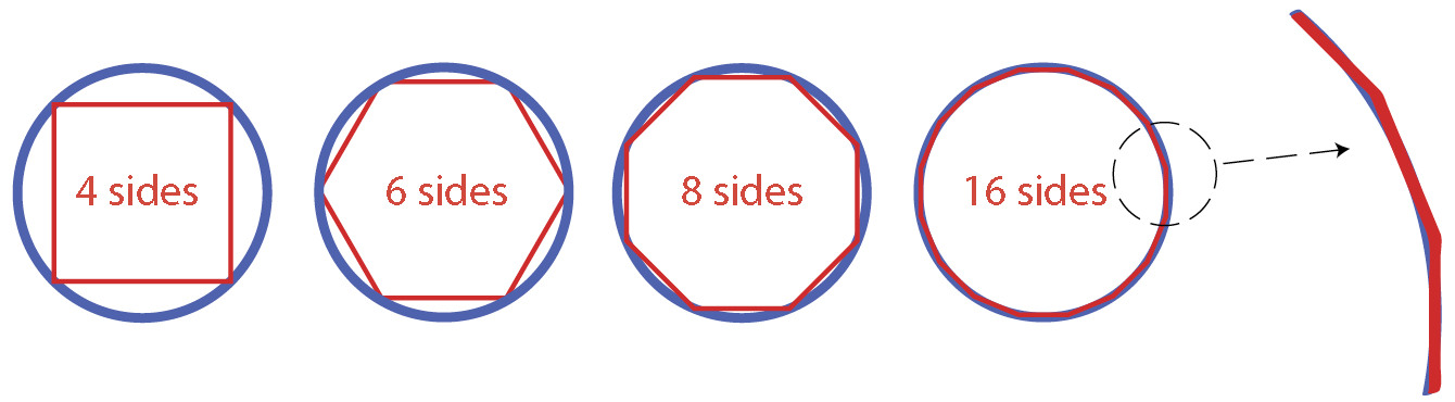
The 'exact' solution
The required exactness of a solution will be project-dependent. In this analogous illustration, the simulation of the visual appearance of the real blue circle by the n-sided regular red polygon has less error (or deviation) as n increases. An increased number of sides requires more calculation work and time, and at some value of n the error is deemed so small that the simulation is considered acceptable; that, in this case, may be when n=16. However, if the image is magnified, to gain greater insight at a particular point, the error may then be unacceptable, so requiring another iteration of the process.
Considering fluids at a microscopic scale, the individual molecules and their associated physical properties – such as temperature, density and velocity – will vary continuously as they move as part of the fluid. CFD takes a higher-level viewpoint that considers blocks, cells or elements of the fluid (which will contain many molecules) and takes averaged values of the individual molecular parameters. So, unlike the somewhat chaotic molecular components, it offers an opportunity to examine the ordered trend of transition and interaction as the focus shifts from one element to its neighbour. The incremental changes between one element and the next will be due to some driving force – such as temperature, pressure difference, viscous forces and gravity. By using the certainty that the whole system will conserve energy, mass and momentum, the interactions between the elements can be evaluated using fluid dynamics.
If this was a matter of examining a single parameter (such as velocity) for a couple of discrete elements in two dimensions – which might be analogous to the collision of two smooth ceramic balls rolling on a polished table top – then it would be possible to examine this analytically, using equations to get a single ‘exact’ solution. However, the challenge soon becomes too complex for simple analytical methods when considering numerous elements while examining multiple parameters in two or three dimensions. In terms of the dynamics of fluids, the Navier-Stokes equations give a set of partial differential equations used to combine the conservation principles and the viscous forces in fluids to mathematically model a flow. Concurrently, heat transfer within the fluid – used to determine temperatures and heat flow – is examined in accordance with the conservation of energy. These methods have been evolved assuming an infinitesimal element of fluid, and by developing sets of differential equations that can be simultaneously solved to determine the required set of parameters associated with the flow of the fluid.
Deconstructing the complex into the doable
To solve a complex, commonplace non-CFD problem, such as creating a building, it is standard to divide it into sections (form, structure, engineering services, and so on) and then further subdivide each of these – an example in engineering services might be internal environment -> heating -> emitter sizing, and so on – until the scale of the challenge makes it possible to solve each element. Then the individual solutions are integrated to make the whole – the building project having been broken into an interconnected mesh of tasks that are interdependent. The effort required to deliver the solutions for each individual element will not necessarily have any direct relationship to the physical size of the space under investigation.
Although there are a few, very simple, laminar flows for which these equations can be solved analytically, CFD software employing numerical (iterative, trial and error) methods are typically used to converge on an ‘exact’ solution (see ‘The exact solution’ box). Many numerical methods have been developed to provide the closest approximations with the least calculation effort, and have been implemented in commercially available CFD software packages.
When setting out to undertake a CFD analysis, pre-processing includes ‘cleaning up’ the building model and converting it into a compatible format so that the geometry may be used by the CFD software in preparation for creating a suitable ‘mesh’. When considering a complex continuum of fluid flow – such as water inside a pipe, or cooled air from a fan coil blowing into a room – the process is far more doable (see the ‘Deconstructing the complex into the doable’ box) when the domain is broken into smaller elements and the velocity, momentum and temperature (and other parameters as needed) are considered in terms of the conditions at the inlet face(s) and outlet face(s) of each element (in two or three dimensions), with no requirement for knowing the detail of what happens within the element.
To analyse and solve the series of partial differential equations that describe the changes across a space, such as a room or an air duct, a contiguous virtual mesh is defined with varying sizes of polygons that completely fit the space. For example, in 2D these might be triangles or quadrangles, and in 3D tetrahedrons, hexahedrons, pyramids and wedges. Zones where there is likely to be a greater rate of parameter change would be broken into smaller elements to provide the finer granularity – for example, adjacent to a boundary formed by a heating coil, or to resolve the smallest flow eddies in an air stream. Where there is likely to be less active change – for example, on the centreline of a straight duct – larger mesh elements would be used. This is to optimise the number of calculations where each mesh element will represent an individual solution of the equation that, when combined for the whole network, results in a solution for the entire mesh. Solving the complete problem without dividing it into smaller pieces can be impossible because of the complexity in the modelled domain, such as holes, corners, curves and angles. Many of the CFD software packages include (or can be linked with) automated and, more recently, dynamically adaptive, mesh generation.
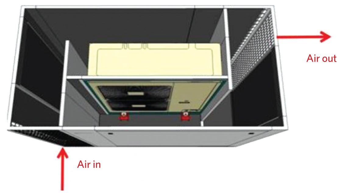
Figure 1: Top view of acoustic enclosure for VRF unit, with top horizontal panel removed (Source: LG)
The numerical approach is employed to solve iteratively across the mesh until the method converges on a solution that practically coincides with the boundary conditions. Boundary conditions are set for a specific set of elements, such as those representing the walls in a room, the coil surface in a heat exchanger, and the velocity and pressures of air streams, which must be physically true to obtain a CFD solution that is properly constrained in the real domain. Missing, incomplete or incorrect boundary conditions will probably prevent a CFD solution. Thermal models can be linked to CFD packages to allow the dynamic variation of boundary conditions resulting from both the CFD output and changes in the building system itself. The solver will approach a solution by the reduction of errors from the previous iterations, with differences between the previous two iteration values providing the error. If the absolute error is descending, the software is said to be converging towards a stable solution where eventually the computed and physical boundary parameters will be practically consistent.
For example, if considering air distribution in a room with air supplied from a diffuser, the velocity of the air leaving the diffuser is a boundary, as is the velocity at a wall surface (that is, zero velocity for air passing through a wall). Accounting for all the boundary conditions, the CFD solver will apply the simultaneous set of describing equations so that after numerous iterations there will be (almost exactly) zero velocity at the wall surface.
An informed initial guess at where to start from (for example, temperature, velocity and so on) can provide an accelerated route to a solution. As with everyday tasks, it is normally quicker if experience, rule of thumb, a template or an inspired guess sets the appropriate starting point (or condition). Otherwise, it can take longer to converge on the most appropriate solution if starting with a ‘blank piece of paper’. Conversely, if the estimated first condition is wildly inaccurate, then the challenge may be exacerbated in the same way as the apocryphal lost traveller who, when asking a local resident for directions, is told: ‘If I were going there, I would not start from here.’ Informed input can be provided with the integrated output of other simulation tools. The CFD software will use one or more turbulence models to most effectively model the system when accounting for flow regimes (such as high-velocity, rotating or separating flows) and boundary characteristics. For example, so called ‘low Reynolds number models’ are used to effectively solve where there are swift changes in the values of parameters close to walls, but these require very high mesh resolutions and so come with a high computational cost.
Traditionally, CFD software employed simple text-based input. This allows extreme control of the input data, as well as benefiting from explicitly knowing what data have been entered. The development of graphical input interfaces – as well as visual output – has enabled access to CFD for those who are not experts in the CFD code. Although, inevitably, this can produce poorly defined models and practically meaningless output, it does allow a wider group of users to develop skills and become accomplished in the application of CFD as a means of exploring their engineering solutions. There are also computer-aided design packages that link directly to, or are integrated with, CFD solvers (with meshing) that may lack the flexibility to examine more specialist applications but provide a potentially swifter path to CFD solutions. The industry-leading CFD packages include sophisticated pre- and post-processors, as well as a variety of solvers – the combination of mathematical formulae and solution methodology ¬ and turbulence models.
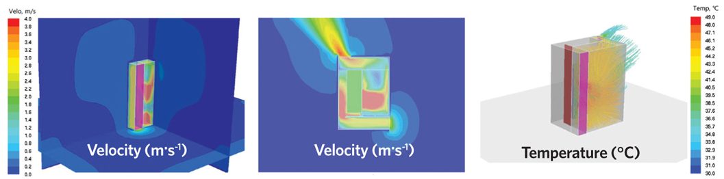
Case A – Original case design. The airflow dropped by 38% compared with a freestanding unit
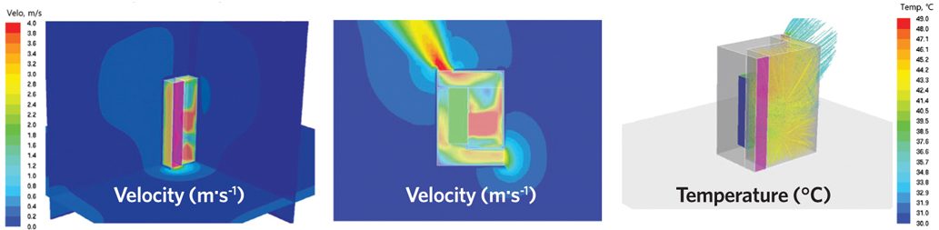
Case B – Inlet perforated panel (on left side) removed. The air flow dropped by 29% compared with a freestanding unit
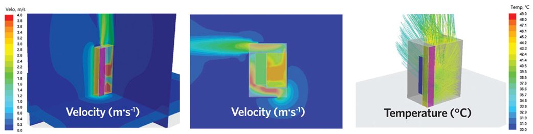
Case C – Inlet and outlet areas doubled with top outlet opened. The airflow dropped by 20% compared with a freestanding unit
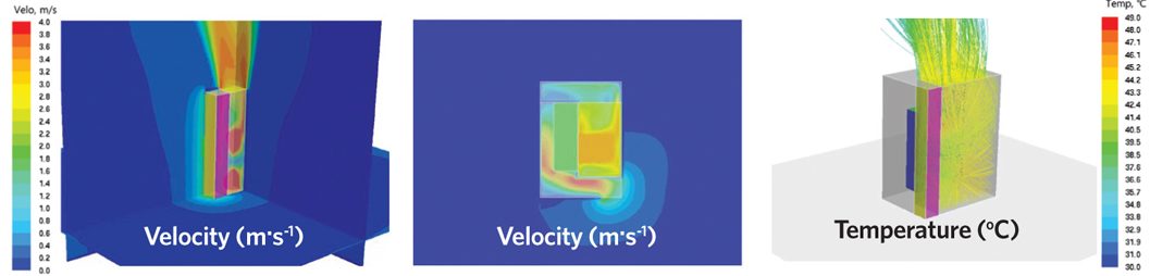
Case D – Inlet areas doubled with top outlet opened and side outlet closed. The airflow dropped by 25% compared with a freestanding unit
Figure 2: CFD analysis of acoustic enclosure for external VRF unit (Source: LG)
Example CFD application
Individual acoustic enclosures were required for a set of outdoor units of a variable refrigerant flow (VRF) system. The inlet and discharge sections of the specific enclosure (as shown in Figure 1) needed optimisation to reduce the emitted noise levels while having minimum effect on the VRF performance. Key control parameters were that the unit must not exceed an operating temperature of 48°C at the heat exchanger, and that the configuration should minimise the short-circuiting of air between the discharge and the inlet. The CFD package allowed for the assessment of the acoustic environment, as well as air temperatures and velocities, so enabling the optimisation and subsequent satisfactory installation of the enclosure.
The output from the analysis is shown in Figure 2. The temperatures and flowrates from the CFD were used to establish the resulting effect on the performance of the VRF units. (This could require an iterative process in itself, as an alteration in the heat transfer in the VRF unit may alter its coil temperature, which would have created one of the boundary conditions for the CFD.) Since there are multiple units mounted together in a line, Case D was selected as the solution, as the air was discharged at the top – this reduced the effectiveness of the VRF unit by 9%. For individually mounted units, Case C might be the preferred option (with a 7% reduction in effectiveness).
The cost of CFD is relatively low compared with the cost of the personnel that will use it and, particularly in commercial applications, the total cost of ownership must include the costs of setup and interfacing. The increased sophistication, usability and intelligence in pre- and post-processing – together with the plethora of free online learning resources – offers great opportunities for many building systems professionals to, at least, become more familiar with the application of CFD.
© Tim Dwyer, 2018.
Further reading:
There are many sources of information available. The following will give a good introduction to CFD:
- What is CFD?
- And this free EdX online course could take you towards being a CFD practitioner: ENGR2000X – A Hands-on Introduction to Engineering Simulations.