
As reflected in the most recent CIBSE Guide B11, the demand for DHW varies greatly depending on building type, but also differs considerably between buildings of the same type. So prediction of DHW consumption and the sizing of DHW systems is a challenging engineering task. However, as buildings become more energy efficient in terms of HVAC and lighting, so the energy consumption of DHW systems increases in significance, and the optimum choice and design of DHW systems becomes ever more important. By applying net present value techniques with simple financial models – together with carbon-impact models – systems can be evaluated and compared, to determine which is the most effective. The sensitivity of the models to the input data – such as assumed hot water demand and fuel costs – can be readily tested to ensure that there is a reasonable degree of confidence in the overall outcome.
As reflected in the findings of a 2011 study of practical water use in ‘sustainable’ homes, ‘there was evidence of occupants exhibiting water-use behaviour associated with practical limitations of low-flow taps: that is, the practice of filling kettles and other kitchen utensils from bath taps’2 – which reinforces the need to consider carefully the assumed input data used in water usage models.
A comparison undertaken by an independent consultant for a continuous-flow hot-water heater manufacturer considered different heating and hot-water supply scenarios for two student accommodation blocks, with a total of 643 occupants, to give comparative 20-year NPV costs and equivalent carbon emissions.
Based on data from the Plumbing Engineering Services Design Guide3, a daily DHW usage profile was created (shown in Figure 1), which equates to a daily usage rate of 70l per person that – in energy terms – is approximately 1,733kWh, based on a 55K temperature rise between the incoming cold water and the heated water. The DHW demand was adjusted seasonally to account for typical student occupancy profiles, while the incoming cold-water temperature was assumed to follow the average ground temperature at a depth of 1.5m. The annual demand for DHW was thereby determined as 536MWh per year, before allowing for storage and distribution losses.
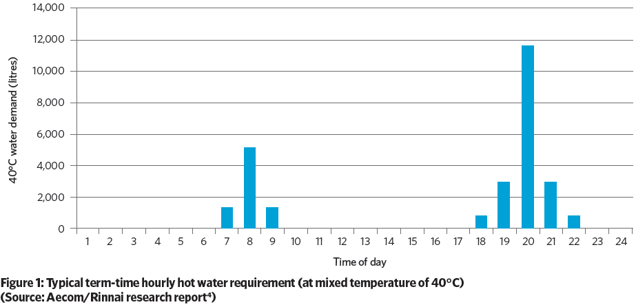
The predicted peak hot-water demand was based on all occupants having a shower within a one-hour period, so each consuming 40l of water – thermostatically mixed from cold and hot water at point of use to 40°C – that equates to a peak instantaneous DHW demand of 4.3L·s-1 (15,480l per hour) at 60°C.
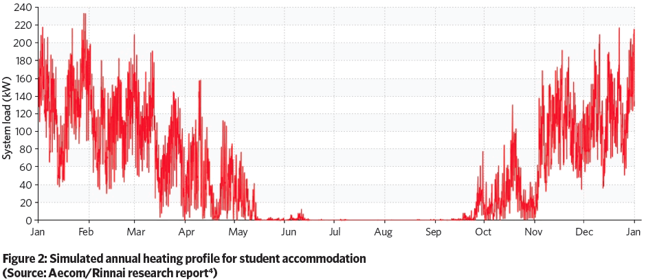
The demand for space heating was determined using a dynamic thermal model of the two student accommodation blocks, and the resulting annual heating-load profile is shown in Figure 2, which equates to 445MWh per year, excluding storage and distribution losses. The simulation applied the CIBSE Test Reference Year (TRY) for London – as described at www.cibse.org/weatherdata – and the building model was created to meet the requirements of the England and Wales Building Regulations Approved Document Part L 2013 for carbon emissions targets and the performance of thermal elements and fittings. Each bedroom has 8l·s-1 of extract ventilation, with 50% of the ventilation make-up air modelled as coming directly from outdoors – via window trickle vents – with the remainder from the adjacent unheated corridors.
A base-case system was established, with two calorifiers providing a total of 37% of the hourly peak load (one 2,900l DHW calorifier in each building), storing water at 65°C with approximately 15kWh daily standing losses. The remainder of the DHW was generated from heat supplied directly from the boiler primary circuit through plate heat exchangers. The recirculating DHW distribution circuit was modelled as returning water at 55°C.
To meet this DHW load, together with a peak space-heating demand of 330kW, the base system comprised a set of modular boilers – located together in one plantroom – delivering a total heat output of 1.44MW (six modules each providing 240kW) with a primary flow of 80°C and return of 50°C. Distribution pipework, insulated to meet the requirements of the UK Building Regulations, had total heat ‘losses’ of 23kW for the DHW pipework – based on 60°C water and ambient temperature of 20°C – and 31kW for space-heating pipework (based on 65°C water and an ambient temperature of 20°C). The heat loss from the pipework was seasonally adjusted for water and ambient temperatures.
Five system configurations were compared to the base case:
1.
Gas boiler LTHW heating + gas continuous flow DHW (no DHW storage) DHW demand met by 18 natural gas-fired continuous-flow water heaters, similar to those shown in Figure 3. The main boiler plant was reduced in size, as it is serving only the space heating (that is, 0.40MW instead of 1.44MW) and there is no storage requirement for DHW.
2a.
Electric space heating + electric DHW (+ DHW storage) Both space heating and hot water are generated using electric resistance heating. As rooms have electric panel heaters, there is no LTHW distribution pipework. DHW is generated by calorifiers with immersion heaters, so requires 100% storage to meet peak demand, which equates to around 15,500l, with approximately 27kWh daily standing losses.
2b. Electric space heating + gas continuous flow DHW (no DHW storage) As per configuration 2a, but where the DHW is provided by 18 natural gas-fired continuous-flow water heaters, with no requirement for storage.
3a.
Air source heat pump (ASHP) heating + ASHP DHW (+ DHW storage) Both space heating and DHW are generated using air source heat pumps. Because of the limited capacity of ASHPs, 100% DHW storage is required. The analysis is based on multiple commercial modular ASHPs, each with an output of approximately 45kW. The LTHW flow temperature and the temperature differential are lower – depending on the ambient temperature, the flow will be between 55°C and 35°C, and the flow/return temperature differential will be 10K. Hence, the flow rate is doubled, compared to the base case, and the pipe diameters are increased by 50%, which also affects pumping energy, distribution-pipe costs and heat losses.
3b.
ASHP heating + gas continuous flow DHW (no DHW storage) As per configuration 3a, but where the DHW is provided by 18 natural gas-fired continuous-flow water heaters, with no requirement for storage.
Each of the systems was designed, modelled and costed. Separating the space heating and DHW allows each system to operate more efficiently. In both the base case and option 1, there are modulating condensing boilers with weather compensation – but whenever there is simultaneous requirement for space heating and DHW, the base case boilers will not operate as efficiently, as the DHW heat exchangers result in higher return-water temperatures to the boilers. The seasonal efficiency of the base-case boilers supplying both heating and DHW is around 89%, compared with the standard seasonal efficiency of the space-heating boilers of around 91%.
The complete ASHP solution (option 3a) has a seasonal coefficient of performance (COP) of around 2.4, compared with 3.1 in option 3b, where the heat pumps are providing only space heating. In this case, the reduction in efficiency is the result of the reduction in COP as the heat pump’s condenser temperature is increased to produce hot water.
The capital costs of the continuous-flow water-heating systems are favourable, mainly because of the saving in the cost of the storage cylinders. They also maintain a seasonal efficiency of around 95%, as they are optimised and controlled to maintain high-efficiency hot-water generation.
The distribution pipework requires a significant capital cost, so the options with electric panel heating have significantly lower capital costs, as there is no need for LTHW pipework. The annual heat losses in the distribution pipework show that the heat loss through the space-heating pipes is between 22% and 25%, while for DHW pipework it varies from 35% to 39%. This would indicate that further savings could be achieved through the approach of distributed – instead of centralised – generation, both in terms of energy and in the capital costs resulting from the omission of distribution pipework.
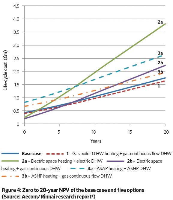
Using the resulting data (the grey-shaded section) from Table 1, a life-cycle comparison was undertaken for a period of 20 years, based on the expected system service life before any replacement. The NPV calculation was based on a discount rate of 3.5% and an inflation rate of 2% for maintenance costs. (See CIBSE Journal October 2016 CPD for an explanation of the NPV method.) The analysis applied projected retail fuel costs and equivalent carbon emissions factors (CO2e) for electricity, based on UK government data.5 Although the equivalent carbon-emission factors for gas would also vary over time, no reliable projections were found at the time of carrying out the analysis, so it has been assumed to be constant at 0.184 kgCO2e·kWh-1, which is taken from the UK government greenhouse gas (GHG) conversion factors for company reporting.
The yellow-shaded section from Table 1 summarises the comparison in terms of 20-year life-cycle cost and operational CO2e emissions. The system with the gas boiler LTHW heating and gas-fired continuous-flow DHW (option 1) has the lowest cost. The operational CO2e emissions over 20 years indicate significant differences between gas- and electric-based heat sources, with the all-heat-pump solutions generating around a third of the CO2e of the base case.
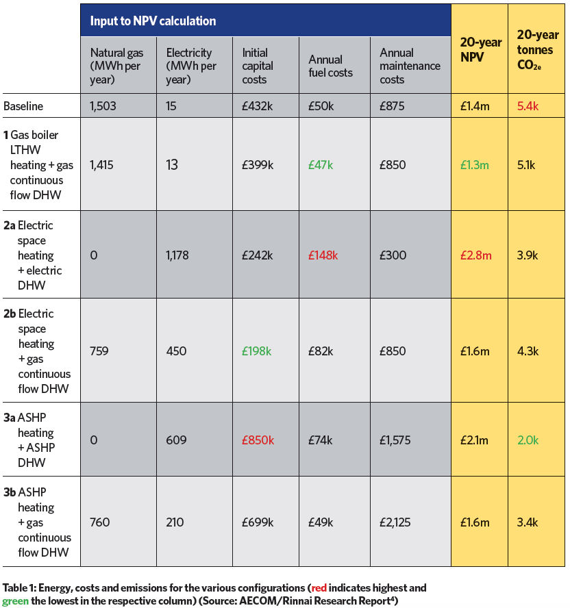
Figure 4 illustrates the discounting effect on capital and operational costs that, in this particular case, indicates that the systems need to be considered for at least five to 10 years before the life-cycle trend is clearly set.
The analysis that is reported in this article indicates that – to establish a reasonable understanding of the total impact of the different systems – some form of whole-life assessment is required to provide a more informed input into the final selection.
Further reading:
The comparison of the systems in this article is based on the output of the independent study undertaken by Aecom on behalf of Rinnai. For more information on the full report, email info@rinnaiuk.com.
References:
- CIBSE Guide B1 Heating, CIBSE, 2016, p.120.
- Water consumption in sustainable new homes, NHBC Foundation, 2011.
- Plumbing Engineering Services Design Guide, Institute of Plumbing, 2002.
- Life-cycle comparison of heating systems – Task 2 – Student accommodation case study, Aecom/Rinnai UK, June 2017.
- CRC Energy Efficiency Scheme Order: Table of Conversion Factors – accessed 1 August 2017.
© Tim Dwyer, 2017