There are several dynamic simulation packages in common use by CIBSE members to assess the heating and cooling loads in buildings. These enable the sophisticated application of computer algorithms to provide an interpretation of how a building will perform but, as with any complex tool, require a relatively high level of resource (information and time) to provide satisfactory results. However, the relative thermal performance of a particular building will depend on a few well-defined parameters. This CPD will explain these parameters (concentrating on opaque structures), and will set the scene for a follow-up article that will apply a simple, freely available tool to explore the need for active building heating and cooling.
In May 2011, the CIBSE Journal CPD article considered variations in thermal transmittance – U value (W⋅m-2⋅K-1) – and, subsequently, in June 2011 considered the effect of non-homogeneity on U values. The U value is determined by summing up the thermal resistances of a structure, with each resistance calculated by thickness, d (m), divided by thermal conductivity, λ (W⋅m-1⋅K-1). However, no matter how well the U value is characterised, it will only provide an interpretation of the steady state heat flow through a structure using the basic relationship Q = U&mulitply;A&multiply;Δθ,where Q is heat flow (W), A (m2) is area of wall/roof through which the heat is flowing and Δθ is the temperature difference (K) between the two sides of the structure.
In the real world, there is rarely, if ever, a time in a building’s life where there is true steady state. For even in winter, where outdoor conditions may be thought to be close to steady state, the building will be exposed to variations in the building occupancy, the radiant solar gains will continue cycling throughout the day and, critically, the building fabric will act to absorb and release heat both from the inside and outside. A reasonably accessible method for approximating the cycling flows of heat and assessing the resulting need for heating or cooling was developed by BRE, and adopted by CIBSE as the ‘admittance method’, more than 40 years ago1. The output of the admittance method is comparable with more sophisticated dynamic computer methods but is inherently limited, as it uses a simplified treatment of loads. For example, when assessing cooling loads, it treats the outdoor daily temperature profile as being constant over a repeating number of consecutive days and, for heating loads, it assumes a constant outside air temperature and no solar gain.
Also, the basic implementation of the method maintains a constant infiltration/ ventilation rate (outdoor air passing directly into the room).
However, despite its deficiencies, the benefits of the simplification from applying the admittance method still holds good even today, where a tablet computer (or a smartphone) can undertake sophisticated numerical analysis and calculate building loads. The thermal admittance method is particularly useful for those designers who are less experienced in building modelling, so that they can gain an understanding of the sensitivity of proposed designs to variations in the basic thermal properties of the construction.
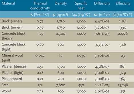
Figure 1: Example thermal properties of materials
Thermal properties that affect building performance
The primary parameters that affect thermal performance of an opaque material are its density, ρ (kg⋅m-3); specific heat capacity, Cp, (J⋅kg-1⋅K-1); and thermal conductivity, λ (W⋅m-1⋅K-1).
The three terms may be combined as thermal diffusivity, α = λ / (ρ⋅Cp) m2⋅s-1, which is an indicator of how rapidly heat is conducted in a material. The depth that the daily changes in temperature reach within the material will depend on thermal diffusivity. So, considering the data in Figure 1, the thermal diffusivity of common materials ranges from about 1.4 x 10⁻⁵ for steel down to towards 8 x 10⁻⁷ for concrete materials. Materials with higher thermal diffusivity values can be more effective for cyclic heat storage at greater depth than materials with lower values.
The thermal effusivity, Β = (λ⋅ρ⋅C )0.5 J⋅m-2⋅K-1s-0.5, is used to present the capacity of a material to absorb and release heat. This relationship is also known as the ‘thermal inertia’. It can be particularly useful when examining multi-layered structures with thin layers. Materials with high thermal effusivity will more readily dissipate heat from their surface, and so will be suitable for storage as well as having a high storage capacity. However, at a surface of a wall or roof there are additionally the convective and radiative coefficients that will more directly dominate the amount of heat transfer. The amount of heat flow will be determined by the surface roughness, shape and emissivity (for radiation) and the speed and turbulence of the air passing across the surface (for convection).
The thermal admittance procedure2 is based around a regular (and theoretical) 24-hour cycle of heating and cooling loads. The fundamental variables in the method may be calculated using an application of the standard non-steady state heat flow equation3 that considers how much heat is stored in, and how much heat passes from, a small element of thickness x (m) of the structure in a time period t (s), in order to determine the change in its temperature, Θ (K). So this can be shown, in classical differential format as:
δθ/δt = α (δ2θ/δx2)
and this is rearranged in CIBSE Guide A3 to be
δ2θ/δx2 = (ρc/λ)⋅(δθ/δt)
To solve this, matrices are applied (see Guide A3 for full details and a worked example). The resulting solution takes the internal and external surface resistances, and applies matrix coefficients to represent each of the layers (m, n…. etc.)
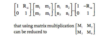
and the four coefficients, M1 to M4, are then directly used to provide the key, non-steady state factors used in the admittance method.
This calculation may be readily undertaken for single layer structures; however, to tackle more than one layer requires lengthy matrix manipulation and is better suited to computer methods (it employs imaginary number notation and can be quite straightforwardly laid out in a spreadsheet, as in the example at http://goo.gl/rxOoF).
The principal values used in admittance method, as derived from the four matrix coefficients, are:
Thermal admittance, Y (W⋅m-2⋅K-1), provides the name for the method itself and is also a key parameter in determining the response of the internal surface of the building fabric to heat. It is a measure of the ease by which energy will pass through the internal surface of the element to, or from, the room per degree of temperature difference between the surface at a particular time and the ‘room’ average temperature (environmental temperature is used to represent the room’s temperature). This is simplified, based on a 24-hour sinusoidal cycling of heat flow into the surface and, in electrical terms, just as the U value is the reciprocal of the total resistance, Y is the reciprocal of the impedance (known as ‘susceptibility’). It is closely associated with the admittance time lead, ω (hours), that provides the time delay between the peak heat flow passing through the surface into the room and the time of the peak room temperature.
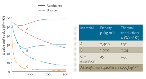
Figure 2: Comparison of U value and admittance for example single skin walls4
As can be seen in Figure 2, the value of thermal admittance is predominantly affected by the part of the wall closest to the room – as the wall increases in thickness, the value of admittance practically approaches a constant value. For very thin walls and those with low thermal conductivity, the U value and Y value are the same. This would be the assumption made for elements such as windows and doors.
Note that the thermal admittance, Y, is completely unrelated to the ‘y-value’ as used as a performance metric for thermal bridging).
Decrement factor, ƒ, is a ratio that accounts for the thermal dampening that reduces the magnitude of the swing in temperature imposed on one face of the fabric as the temperature wave passes through the structure – the effect of which is shown in Figure 3. And the time lag, φ (hours), is how long it takes for the heat passing into one side of a structure to get to the other side (and, of course, the magnitude will have been reduced, due to the decrement factor). So, for example, the careful selection of materials can ensure that high solar irradiance striking the outside of a wall is not felt inside the space until after the building’s use has ended for the day.
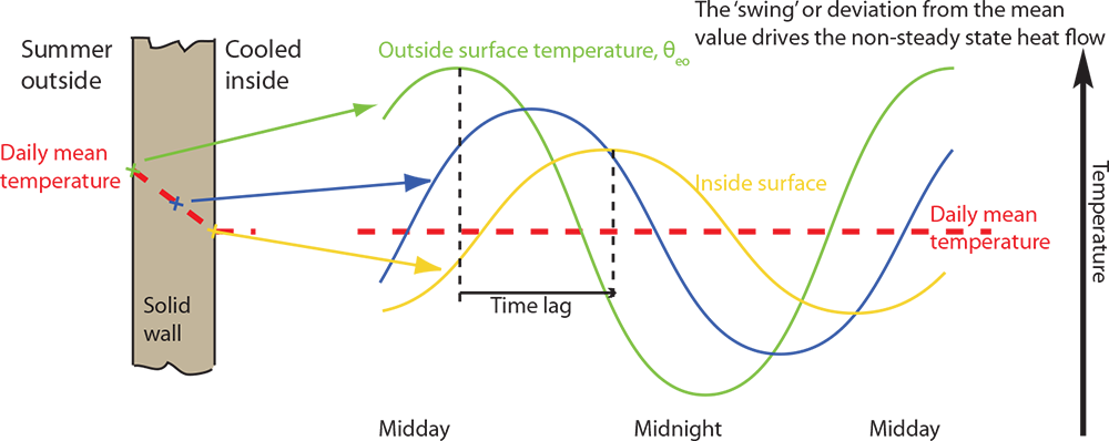
Figure 3: Daily temperature profile at points through a concrete wall
The final pair of factors are Surface factor, F, that is the ratio of the swing in heat flow from the internal surface of the element to the swing in heat flow received at the internal surface of the element (such as the gain from localised sunshine through a window), and an associated time factor, ψ (h), that defines the time delay.
Calculated admittance data for some example constructions are given in Figure 4. For example, comparing the external walls (A, B and C) clearly shows the impact of the structures to improve the heat loss (by reducing the U value) can make significant alterations to the admittance and decrement factor that may adversely affect the resulting room cooling loads. The selection of internal walls (for example, D, E and F) can make a major difference to the average room admittance.
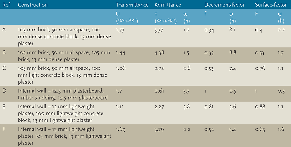
Figure 4: Thermal properties of example constructions taken from the CIBSE Guide A3 (the external constructions are not suitable for modern buildings – used for illustration only)
If seeking out a particular thermal admittance value that is not specifically listed in the CIBSE tables, it should be possible to find a similar structure as an approximate proxy, considering that the admittance is normally defined by the characteristics of the inner 100 mm of the surface (or, better still, the value can be determined using a spreadsheet).
Published values of thermal admittance are calculated on a basis of sinusoidal variation of heat input and temperature. In practice, these conditions rarely occur. Theoretically, it would be possible to calculate thermal admittance of periodic conductance for any pattern of heat gain, but to retain the simplicity of a thermal admittance method, standard thermal admittance values are generally used.
The follow-on CPD article will apply the thermal admittance method to undertake some concept ‘what-ifs’ to help reduce the heating and cooling loads.
© Tim Dwyer 2012
Further reading:
See the relevant appendices CIBSE Guide B3 and CIBSE Guide A5 – they are a mine of information.
References:
- Loudon, A.G., Summertime temperatures in buildings without air conditioning, JIHVE, 1970.
- CIBSE Guide A3, Appendix 3.A6, CIBSE, 2006.
- Rogers and Mayhew, Engineering Thermodynamics, Work and Heat Transfer, Prentice Hall, 1992.
- Millbank, N.O and Harrington-Lynn, J., Thermal response and the Admittance Procedure, BRE CP 1/74. BRE. 1974.