The reduction of energy use in buildings is not only an economic issue but also increasingly linked with opportunities to lessen the demand on the primary energy source (and distribution networks), as well as reducing life cycle environmental impact. This CPD article will consider heat recovery in mechanical ventilation systems using plate heat exchangers and show how to compare annual heating performance using binned weather data.
Heat recovery systems
Heat recovery in HVAC systems will typically exchange heat between the discharged room air and that being introduced from outdoors. The system may be designed to exchange only sensible heat or both sensible and latent heat. Details of the principal system types may be seen in Section B of the CIBSE Guide.
An example of a sensible heat recovery process is shown in Figure 1.
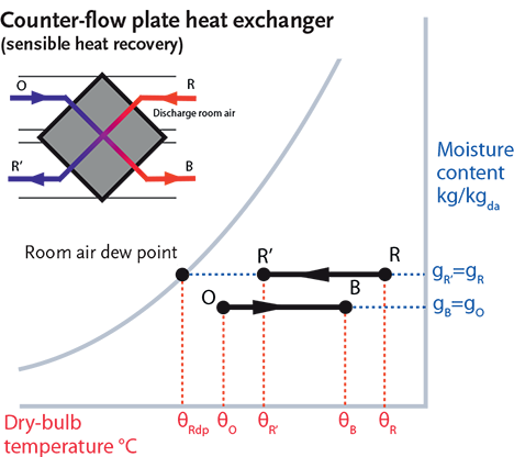
Figure 1: Psychrometry of cross-flow plate heat exchanger
This psychrometric process indicates an increase in the sensible heat of the incoming air that could take place in a cross-flow plate heat exchanger, a (regenerative) thermal wheel or a run around coil. The process is a basic sensible heating or cooling process – depending on the temperature of the opposing airstreams.
The heat exchanger sensible heat effectiveness, εS = ṁO(θB – θO)/ṁR(θR – θO), where ṁO and ṁR are the respective air mass flow rates of air at outdoor temperature θO, θR the room temperature, and θB being the temperature of the outdoor air after is has been through the heat exchanger.
Considering Figure 1, if the temperature of the incoming air, θO, is below the dew point temperature of the extracted air, θRdp , there is likely to be some condensation in the airstream that is coming from the occupied space, so providing increased heat exchange. But, in the case of a simple impermeable plate heat exchanger, there is no transfer of water vapour. The heat Figure 2: A section through a combined counter- flow and cross-flow plate heat exchanger of condensation will add to the recovered heat. In recent years, the simple cross-flow plate heat exchanger has been developed to provide an additional counter-flow component, as illustrated in Figure 2.
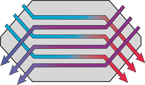
Figure 2: A section through a combined counter-flow and cross-flow plate heat exchanger
Owing to the extended heat exchange surface, the effectiveness is increased (as is the air side pressure drop). The manufacturer1 reports a seasonal sensible heat exchange effectiveness of 85%; such a process is illustrated (approximately) in Figure 3, where the condensation from the discharge air further increases the dry bulb temperature of the incoming outdoor air.
The additional resistance to air flow will require energy for fan power (W) given by:
Power = Q⋅ΔΡ/ηfan
where Q is the air volume flow (m3⋅s-1), ΔΡ is the additional pressure drop through the device (Pa) and ηfan is the total fan, drive and motor efficiency. This will be additional direct electrical power, which is likely to be more costly – and have twice the carbon footprint – of any natural gas heating that is being offset or any cooling savings (owing to the coefficient of performance (COP), refrigeration electrical power consumption will typically be less than half the cooling delivered). The heat recovery device will also require a bypass to avoid unwanted heat transfer to the incoming air in summer conditions.
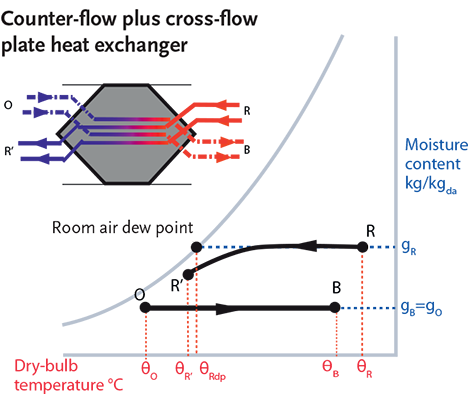
Figure 3: Plate heat exchanger with condensation in the discharging room air
Application of heat recovery model
In this CPD module, a simple example building will be used to examine the impact of heat recovery in a very common application of ventilation in the UK (with no cooling). This is an example of a comparative method that may be used – it can be quickly developed in a spreadsheet that can readily be expanded to explore other sensitivities, including NPV analysis. The building is a small, detached store 20m wide, 10.2m deep and 3m floor-to-ceiling height, situated adjacent to a busy road on the outskirts of London. The building has triple-glazed windows (and doors) along 50% of the long south-facing wall, and has been constructed within the last two years.
The heating and ventilation air is being provided by a mechanical ventilation system to maintain a minimum temperature of 21°C. The occupancy will be one person, 24 hours a day, and the lighting provides a heat gain of 10 W⋅m-2 floor area, with no other equipment use. Owing to the materials stored in the building, full fresh air ventilation is required at a rate of at least six air changes per hour. The building’s data required to undertake heat loss calculations are given in Table 1.
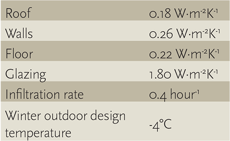
Table 1: Example building data
A heat recovery system is often incorporated into packaged air handling units similar to that shown in Figure 4, designed for mounting in ceiling voids.
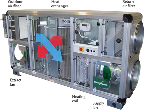
Figure 4: Plate heat exchanger with condensation in the discharging room air
To examine the building and the application of heat recovery in detail requires a dynamic simulation package. However, by using binned outdoor temperature data together with the building heat loss coefficient and assumed casual gains, a reasonable comparative study may be undertaken. The outdoor temperatures for the suburbs of London (hourly data measured over 20 years) is given in the first two columns of Table 2. This type of data can be readily obtained for most global locations from local meteorological offices.
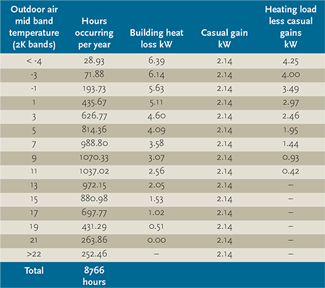
Table 2: Frequency of outdoor air temperature for London suburb (24-hour, hourly data) together with building heat loss at mid band temperature, casual gain and resulting banded heating load
The basic building heat loss coefficient2 may be determined from:
Σ(AU) + Cv = Σ(AU) + 0.33NV = (20.0 x 10.2) x (0.18 + 0.22) + (10.2 + 10.2 + 20.0 + 10.0) x 3 x 0.26 + 10 x 3 x 1.80 + 0.33 x 0.4 x (20.0 x 10.2 x 3.0) = 255.7 W⋅K-1
where A = element area (m2), U = U value (W ⋅ m-2K-1), Cv = ventilation conductance (W ⋅ K-1), N = infiltration rate (hour-1) and V = volume of space (m3).
Using the heat loss coefficient, the building heat loss at each band is evaluated from:
(Σ(AU)+Cv) x (θR – mid band temperature).
The casual gain is shown as a constant at 2.14 kW (comprising the lighting gain plus one person), and this will offset some of the need for heating throughout the whole heating season. When undertaking such an analysis, there would normally be a diversity factor estimated to account for variations in such things as occupancy, lighting and equipment. The final column of Table 2 shows the heating required in the room at each corresponding band of outdoor temperature.
For each band, the required supply air temperature, θS, may be calculated from:
Heating load = ṁ Cp (θR – θS) where Cp is the specific heat capacity of air, 1.005 kJ kg-1K-1. The approximate mass flowrate of air (in this particular case) is determined by the required ventilation rate of six air changes per hour (and taking the specific volume of air as 0.83 m3kg-1) so ṁ=6x(20.0×10.2×3)/(3600×0.83)= 1.22 kg s-1
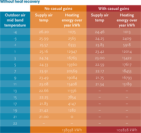
Table 3: Ventilation heating energy with no heat recovery
The resulting supply temperature (both with and without allowing for casual gains) is given in columns two and four of Table 3. The sum of the energy used over a year (relating to each band) is then calculated from:
Hours occuring per year x ṁ CP (θS – θO) where θO is the particular outdoor air mid band temperature. These are then summed to give the total ventilation heating energy used per year – so, in this case, with casual gains being taken into account, this would be 102,828kWh for a full fresh air system.
Having established a base case (illustrated in Table 3) the impact of adding a heat recovery device may be assessed, as in Table 4.
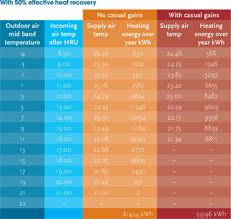
Table 4: Ventilation heating energy with 50% effective sensible heat recovery
As the supply and extract mass flow rates are equal, the temperature of the outdoor air leaving the device, θB, which enters the subsequent heating coil, may be determined from:
θB =θO +εS (θR – θO)
where θO is the particular outdoor air mid band temperature. This has been undertaken for a heat recovery effectiveness, εS, of 50% and is shown in column two of Table 4. (The 50% figure is representative of the seasonal efficiency of an average cross-flow plate heat exchanger.3)
The sum of energy used over a year (relating to each band) is then calculated, but this time only requiring heating from θB to the supply temperature, θS.
The additional fan power (Wh) required to overcome the resistance of the heat exchanger and the additional return air filter may be calculated from:
(Q⋅ΔΡ/ηfan) x hours of operation.
For the cross-flow heat exchanger, a pressure drop of 100Pa (for each of the flow and return paths) is typical, and a panel filter would add 30Pa. The total fan efficiency is related to the fan type and the motor/drive mechanism – in this example, a value of 70% has been used although direct drive EC motors can approach 90% as may be needed to meet regulatory Specific Fan Power requirements.
So additional annual energy use = (1.02 x (100 + 100 + 30)/0.7) x 8766/1000 = 2938 kWh. This will be electrical power, whereas the savings in heating energy could be savings in gas or electricity (or other fuels), depending on the method used for heating on site.
The combined counter-flow/cross-flow heat exchanger can be examined in exactly the same way as the cross-flow but with the efficiency amended to 0.85 (85%) and the pressure drop increased to 150Pa. The results from that analysis, together with the others, are summarised in Figure 5.
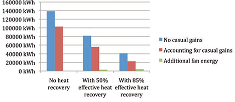
Figure 5: Summary of annual heating energy supplied by ventilation systems and additional fan energy required to overcome heat recovery device resistance
The annual energy consumption may be used to provide a simple approximate cost saving (in terms of heating energy less the additional fan energy), as shown in Figure 6. A similar exercise could be undertaken to show notional CO2 saving.
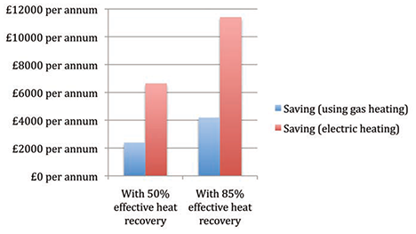
Figure 6: Approximate cost savings applying heat recovery for a system that uses gas heating and one that uses electric heating
It is important to note that this simple model is based on a 24-hour-a-day application with low casual gains. In other applications of 10-hour working and higher occupancies and equipment loads, the savings will not be so dramatic. The application of a compliance tool such as SBEM or, preferably, dynamic modelling software, together with independently certified performance data, will provide a more complete picture of the whole life impact of a heat recovery device.
Appropriately applying this simple technology can increase flexibility in building design, while still meeting rigorous carbon targets. The size of associated heating systems may also be reduced, saving on both capital and installation costs.
© Tim Dwyer 2012
Further reading:
- Air Conditioning Engineering, Jones WP, Butterworth 2001, Section 6.6.
- ASHRAE HVAC Handbook 2008, Chapter 25.
- CIBSE Guide B, Section 2.5.6, 2005.
References:
- Fisher, J., Reducing your Total Building Emissions using High Efficiency Energy Recovery, FläktWoods, 2012
- CIBSE Guide A, Section 5.6.2, 2006
- CIBSE Guide F, Section 5.2.5.5, 2012