The function of the fan is to move the required air flow rate through the system, and to overcome the total pressure loss (the sum of the static pressure losses through the duct system plus the discharge velocity pressure). So when selecting a fan it should be chosen on that same basis – a design flow rate and a total pressure.
The characteristics of a fan are normally obtained from a manufacturer and these would have been based on standard tests measuring the output of a fan – volume flow rate and pressure – for a range of conditions. This is shown (in concept) in Figure 1, ranging from the flow being fully closed off when the air path is completely open – all this at a constant fan speed. At the same time, the power input to the fan (not the motor) is recorded (using mechanical or electrical means).
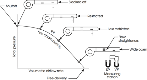
Figure 1: The creation of a fan curve (after ASHRAE HVAC Handbook 2008)
The fan total pressure is made up from the fan velocity pressure – the kinetic energy at the fan outlet (given by 0.5 ρ c2) – and the fan static pressure. The static pressure is wholly available to overcome the pressure drop in the attached ductwork, whereas the availability of the velocity pressure will depend on the velocity at the outlet – if the outlet is the same size as the fan outlet area, then all of this velocity pressure will be lost when the air leaves the system. However a lower final outlet velocity (for example through a diffuser) will allow some of this velocity pressure to be ‘usefully’ employed. Some manufacturers are not clear in catalogue data for their fans, whether the fan characteristics represent total or simply static pressure. The data will reflect ideal test conditions – such as that given in BS5801:2008i. These perfect conditions are unlikely to be matched in practical installations where the challenges of fitting fans into systems introduce bends or other obstructions near the fan inlet or outlet – these will reduce the fan’s performance.
Using the test data, a complete set of fan characteristic curves may be produced as illustrated in Figure 3. This includes the fan efficiency curve that has been produced by dividing air power (pressure, Pa x volume flowrate, m3/s) by the shaft input power. The actual shape of the curves will depend on the type of fan (and the shape of this example is typical of a ‘backward curved centrifugal’ fan). The manufacturer will often identify a ‘selection range’ that is recommended for the fan. This is shown as the yellow highlight in Figure 3.
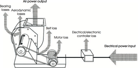
Figure 2: Losses from the whole fan subsystem (after BS 5801:2008)
The fan efficiency varies across the operational range of the fan. The losses will be due to friction in the fan case; turbulence and ‘shock’ losses; losses in bearings and seals; and leakage and shortcircuiting. The total losses (including the whole subsystem from electrical power compared to the air power being supplied) will be somewhat greater than those indicated on the fan curves due to external losses, as illustrated in Figure 2 for an example fan.
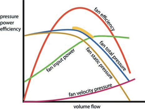
Figure 3: Full set of fan characteristic curves
The fan meets the system
As discussed in recent CPD articles, if the volume flow rate in the ductwork is varied the pressure loss will be related to the square of the volume flow rate. This may be simplified to Δp = RQ2 where Δp is the system pressure drop (Pa), Q is the volume flow (m3/s) and R is a constant for the system relating to its resistance to air flow (the term resistance, should not be confused with system pressure drop).
Using a calculated pressure drop at any particular flow rate, the value of R may be determined and then a curve drawn for a range of volume flow rates against pressure drop, as in the system curve in Figure 4.
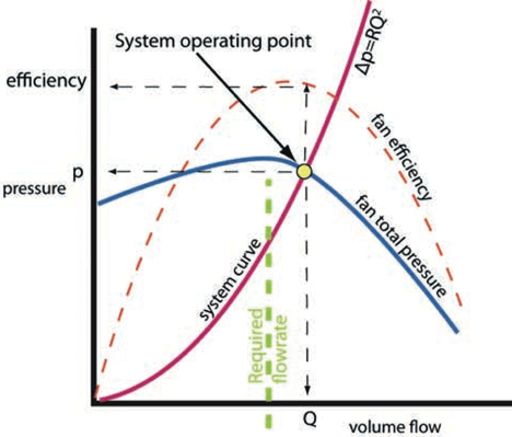
Figure 4: System and fan operating point
This figure has also had the fan curve from Figure 3 superimposed – the fan curve being a series of points at which the fan can operate at a constant speed. Likewise, a system curve is the series of points at which the system can operate. The operating point for the fan-system combination is where these two curves intersect, and this provides the flow rate for this particular fan running at a particular speed with this system. In this case the efficiency also appears to be almost at a maximum so the fan will be operating at its most effective.
However, of course, this is not the required design flow rate (shown in green) – the fan, running at this speed, will deliver more air though the system than is required. Also the practicality of real system operation must not be forgotten. Although the system curve has been established from design calculations, the installed system is bound to differ from this due to installation vagaries and uncertainties in the design data. Also, while in use there will be continuous changes in the pressure profiles, both in the system and the building, so when considering the operating point, thought must be given to the potential range of conditions and the effect they may have on the fan output. The extremes of operation can be particularly significant when considering variable air volume (VAV) systems.
The temperature of the air passing across a fan will affect the mass flow rate of the air. For example, if a fan is simply passing fresh air through a system, then as the external temperature increases the air density will reduce and hence the mass flow rate of air will also reduce. This is shown in Figure 5 – note how the volume flow rate will remain constant.
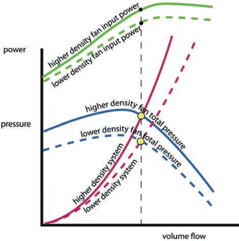
Figure 5: The effect of varying air density of fan and system operation
A family of fan curves
The performance of fans is determined by a number of relationships (known ‘fan laws’) that can be derived to examine what will affect a fan’s operation. In the ranges that would be expected in building services applications:
Q is proportional to D3 N p is proportional to D2 N2 ρ Power is proportional to D5 N3 ρ Where D = fan impeller diameter, ρ = density of air and N = speed of fan rotation
So the flow rate will alter with the cube of the impeller diameter, (and the pressure with the square of the diameter), so a change in a fan diameter will make a disproportionate alteration to the volume flow (compared with the swept area of the fan impeller). And the power (being the product of pressure and volume flow rate) will increase to the fifth order of the diameter, so a small change in fan diameter can produce a large increase in fan power and a consequent increase in motor power and supply electrical power.
The fan’s diameter, D, and the air density, ρ, are normally assumed to be constant when considering a specific fan and system combination, and so the three relationships are conveniently simplified to Q ∝ N, p ∝ N2, and Power ∝ N3. So, for example, a 10% increase in fan speed means a 10% increase in air volume flow rate, a 21% increase in pressure and a 33% increase in power consumption.
And using these relationships families of fan curves can be drawn for operating the fan at different speeds as in Figure 6 – each of the fan speeds has its own operating point with the system but, in this case, only the low fan speed provides the required flow rate for this example.
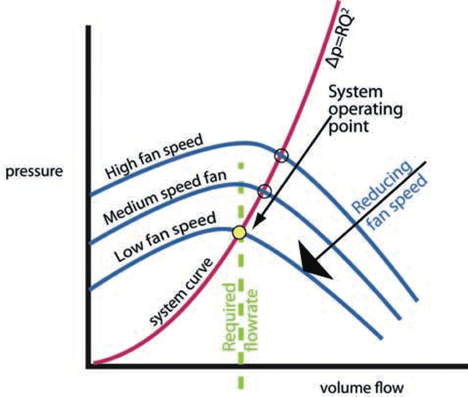
Figure 6: Variable speed fan providing operating point at required flowrate
Varying the flow
The flow can also be altered (reduced) on the system side by adding restrictions (such as dampers) or by altering the way that air is fed into the fan using ‘guide vanes’ or ‘throttling discs’. Although these may be a capitally cheap option, and appropriate for infrequently used systems or for those where only minor regulation is required, their use for significant alterations to the operating point should be carefully considered as they are likely to severely reduce the potential savings available from the reduction of air volume flow rates. Multiple speed electrical motors can be used to provide efficient ‘step changes’ in fan output – this is where there are separate windings within a single motor that can be used to alter the speed to meet specific load requirements (for example, in a cooking area where there are quite different air supply requirements when preparing food, compared to when cooking is taking place). So aside from altering the mechanisms or the physical size (or possibly geometry) of the fan, the increasingly adopted option is to alter the fan rotational speed. This would have traditionally been undertaken through mechanical devices such as hydraulic clutches, fluid couplings, and adjustable belts and pulley. (Altering pulley sizes on indirectly driven fans is still routinely used as an efficient way of setting a fan’s installed speed.) Electrical devices have also been used, such as eddy current clutches (where the torque passed from the motor drive to the fan is varied) and wound rotor motor controllers (where motor voltage or resistance is altered). More recently variable frequency drives, VFDs (often known as ‘inverters’), have become a cheaper alternative.
VFDs vary the effective supply frequency to the AC fan motor giving speed reductions down to 20%. The power conversion efficiency of such drives is typically above 96%, although the imperfect output waveform created by the electronics (ie not perfectly sinusoidal) may reduce peak motor efficiency by 1 or 2%. Motor efficiency may itself reduce significantly at speeds below 75%ii.
When the fan speed is reduced, the curves for fan performance and power both move downwards and to the left. Since the fan efficiency curve shifts to the left as the speed is reduced, the fan can still maintain high efficiencies (as in Figure 4) even at lower output.
Since the principal element of noise from a fan outlet is due to its aerodynamics, reducing the fan speed will mean that the noise emitted by the fan is also likely to reduce. This will then lessen the adverse effects of the ventilation system on occupants and may also reduce the need for sound attenuation. (Note that when comparing two different fans, a slower fan will not necessarily be quieter – the octave band sound power levels of the individual fans at the design flow rate and pressure must be used to compare the noise).
The fans
There are two principal types of fans used in building services engineering for ducted systems – centrifugal and axial. A future CPD article will consider the details, variants and application of these fans and reflect on how installation will affect performance.
© Tim Dwyer 2011