

When air conditioning and ventilation systems are designed, there are often assumptions made that the airflow rate delivered through the ductwork system will match the design intent. However, this is not likely to be the case, leading to inefficient or ineffectual ventilation. This CPD article will consider the methods and practicalities of measuring airflow, specifically concentrating on applications of continuous monitoring.
The opportunity for continuous airflow measurement
It is only in cases where there are specific – and possibly special – needs to monitor the air flow rate continuously that there would normally be permanent air volume flow rate monitoring devices. This would often be where a particular air volume flow rate or room air pressure (normally as a means of maintaining positive movement of air and contaminants) must be assured to meet varying laboratory ventilation or process needs.
However, the challenges of supplying sufficient outdoor air proportions are not restricted to laboratory or process use. Variable air volume (VAV) systems are notoriously demanding to design and operate to ensure optimum outdoor air fraction, as individual zones vary their demands on the total supply air flow rate. Actively monitoring volume flow rates in the outdoor air inlet duct together with zone flow rates provides information for the control system to properly modulate the outdoor and recirculation air fractions. Such control may be driven by the needs of extract systems where variable flow fume hoods are being used. In this case, there is not only a requirement to maintain appropriate total supply flow rates (and resulting room pressures), but also the most energy efficient fresh air proportions in the variable volume supply air to the room where the fume hoods are located (see CIBSE Journal CPD, October 2013, for further details of variable volume fume hoods).
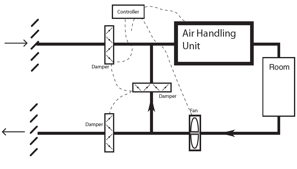
Figure 1: Simplified recirculation ‘economiser’ system
Alternatively, and more generally, accurate airflow measurement can provide essential real time information for the commonly used systems such as the recirculation air system shown in Figure 1.
The system, known as an economiser system, will only properly economise if appropriate volumes of outside air are mixed with the recirculated air – the proportions being set by the indoor and outdoor temperatures (or by comparing enthalpies or possibly moisture contents) and the required amount of fresh air. Without a direct measure of the incoming air volume flow rate, it may take some time – in some cases, many years of operation – before, for example, a poorly performing damper or a faulty actuator is discovered. This could result in long-term inefficient operation. This may manifest itself as in the simulated data in Figure 2 for an economiser system.
The actual flow rate through the outdoor air intake can be adversely affected by such common phenomena as varying outside outdoor wind velocities; stack induced flow within the building altering the building’s pressure profiles; obstructed air intake and discharge louvers; frosted air filters; malfunctioning dampers/actuators; and faulty control loops.
Beyond the day-to-day operational needs when the building has a change of use, a variation in occupancy, altered indoor environmental quality demands or undergoes a refurbishment, real time air flow rate measurement (through both main ducts and individual sub-networks and branches) can enable the building operator to obtain information to inform the recommissioning of the system to satisfy new operational conditions.
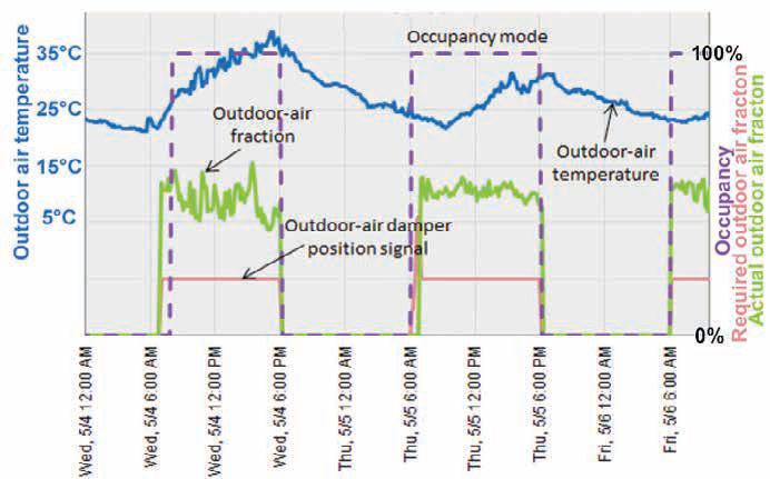
Figure 2: Example of poor performance of outdoor air regulation. The ‘required outdoor air fraction’ should be matched by the ‘actual outdoor air fraction’, but the actual airflow is significantly higher – possibly due to a faulty damper assembly (Based on material from PNNL training document1)
The streamlines of ducted airflow
When air passes through a duct – whether it is rectangular or circular in section – it does not have a uniform velocity over the cross-section of the flowing air, but will have a ‘velocity profile’. The profile will depend on the upstream and downstream ductwork, its roughness and shape, and the qualities of the air. For example, as discussed by Legg2, if an airstream enters the duct through a smooth intake – as in Figure 3 – the velocity profile will develop as the air flows through the duct (the length of the arrows is proportional to the average velocity at that point). It is not until some distance down the duct – possibly greater than 30 times the diameter of the duct with a smooth intake, somewhat less if the intake is more abrupt – that the flow will be ‘fully developed’.
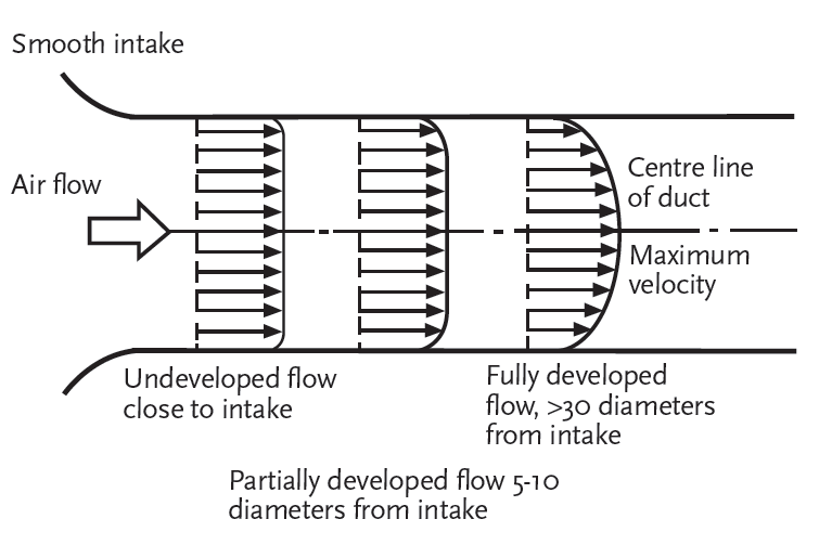
Figure 3: Development of air flow regimes in a ducted air system with conical inlet. The length of arrow is proportional to the average velocity at that point (Source: Legg2)
Although air is often shown schematically as flowing in a set of parallel streamlines (as in Figure 3) that may infer to some that it is ‘laminar flow’, the typical velocity of the air in an air distribution network will determine that the flow will be ‘fully turbulent’. This means that although the bulk of air is moving forward at an average velocity, there is a continuous eddying and mixing within the airflow. Reynolds number (Re) is used to characterise the flow regime. Reynolds number is a ratio of the inertia of a fluid to its viscosity – as the ratio increases, the viscous forces will be overcome by inertia and the air will be able to more readily move around, independent of the adjacent air molecules. A Reynolds number value in excess of 4,000 would typically confirm that the flow is turbulent, and this is the normal situation in HVAC ductwork (see example calculation in box, above right).
Such a turbulent regime will have a ‘flatter’ velocity profile than that of a laminar flow, since the air is moving in all directions – while generally moving forward – so reducing the variations in streamline velocities across the duct. Due to the shear stresses of the air at the wall of the duct (where at its closest the air is practically static) there will be a steep increase in velocity between the turbulent air moving down the duct and the duct wall.
Methods of measurement
The principal measurement techniques for permanent devices are based on basic principles that relate the cross-sectional area, A (m2), of the duct and the velocity, c (m·s-1), of the travelling air to determine the volume flow rate, q (m3·s-1), simply from q = A x c. The actual measurement of the air velocity will be achieved either by using a measurement of pressure drop across a device, or determining another secondary parameter that enables the velocity to be determined.
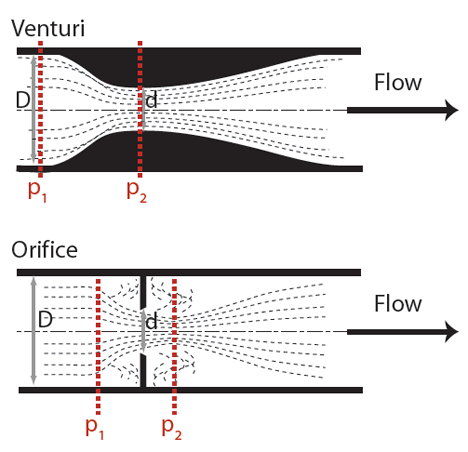
Figure 4: Simplified sketches of orifice plate and venturi measuring devices
Pressure drop method of determining air volume flow rate
Any obstruction in an air stream will cause a pressure drop in the flowing air, due to the frictional resistance and turbulence.
By characterising the obstruction and calibrating the pressure drop against known flow rates, the value of pressure difference may be used to determine the air volume flow rate. For ducted air systems, such measuring devices include venturis and orifice plates – as shown in Figure 4.
Considering the example of the orifice plate, as shown in Figure 4, the volume flow rate of the air may be readily obtained from the differential pressures measured across the two tappings, by combining the continuity equation A·c = constant and Bernoulli’s equation p/ρg +c2/2g = constant (assuming the ductwork is level) where p is pressure (Pa), ρ is density (kg·m3), g is gravity (9.81m·s-2)
This is used with a flow (or discharge) coefficient, Cd, that relates to the energy lost as the air passes through the constriction (that is dependent on the Reynolds number and design of orifice), and the expansibility of air, ε, (that is practically 1 for ventilation air ductwork applications).
So for an orifice plate of diameter d (m) that is installed in a duct diameter D (m) (and the ratio ß = d/D) with pressure measurements p1 and p2 (Pa), the volume flow rate, Q (m3·s-1), can be obtained from Q = Cd ·ε ·π·d2/4 · 1/√ (1-ß4) ·√[2(p1 – p2)/ρ]
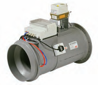
Figure 5: A commercial venturi for ducted air flow measurement close-coupled to a control damper (Source: CMR Controls)
This relationship, although relatively straightforward, is simplified in its application to operational HVAC ductwork, as most of the parameters are fixed or vary little in the normal range of air temperatures (and pressures). So a measuring device (such as an orifice plate) will be calibrated by the manufacturer and will normally be supplied with a single coefficient that, when applied to the pressure drop, will provide a direct value of volume flow rate.
The same fluid flow principles apply to venturi devices. There have been many developments of the simple venturi since the original devices, which were relatively long and expensive. Modern devices used in ducted air systems (as in the example shown in Figure 5) are robust and very low maintenance, and have a length similar to the outside diameter of the ductwork.
The pressure drop as seen by the system (adding to the power demands of the fan and known as ‘permanent loss’) will be somewhat less than the measured (p1 – p2) across the device, as there will be a recovery of (static) pressure as the air velocity reduces following the constriction. For an orifice plate, this may be in the order of 70% recovery (worsening with decreasing value of ß), and a venturi will recover at least 90% (as there will less turbulence) – so, in practice, the permanent losses will be relatively small with a venturi-based device.
Pitot tube devices
A classic pitot-static tube, as shown in Figure 6, is made of two concentric steel tubes with an outside diameter of approximately 10mm.
It measures two pressures – the static pressure, ps, that is measured at right angles to the direction of flow through the outer tube (preferably in an area of low turbulence) and the total pressure, pt (also known as the impact pressure), measured through the ‘nose’ of the inner tube that is open ended and facing directly into the oncoming air. Since the total pressure at a point in a fluid is the sum of the velocity pressure, pv, and the static pressure, so pv = pt – ps and from this, the air velocity may be obtained as pv = 0.5·ρ·c2
If pitot-static tubes are made to appropriate ISO standards, they will not require any calibration coefficient, and so the velocity of the air may be directly obtained at a single point in the duct from c = √[2 (pt – ps)/ρ]
However, as noted earlier, the velocity varies across the cross-section of the duct so to determine an average velocity, multiple measurements need to be taken. The required positions for measurement have been established in numerous standards and, specifically for commissioning purposes, are clearly illustrated in BSRIA Guide to Commissioning Air Systems3 for a ‘pitot traverse’.
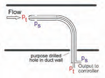
Figure 6: Basic pitot-static tube measurement of airflow
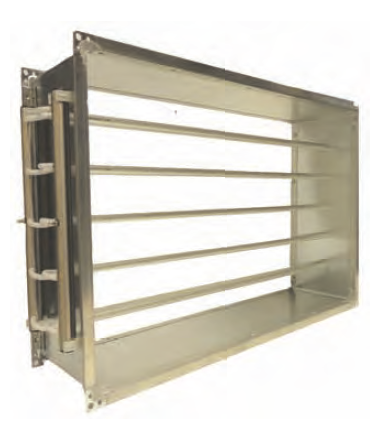
Figure 7: A commercial velocity grid (Source: CMR Controls)
To enable this in a permanent application, frameworks of measuring points have been developed (known as velocity or flow measurement grids) that take measurements across the whole face of the ductwork, as shown in Figure 7. The measuring points are distributed to ensure a representative average velocity sample.
Such grids are likely to measure total pressure and static pressure separately, using appropriately orientated holes drilled into sets of sampling tubes. Velocity grids will be supplied with their own calibration factors to convert the measured pressure into velocity or volume flow rates. They have a significant advantage over single measurements, as they can produce a much higher pressure signal, providing a greater resolution and so feasibly less error – giving measuring accuracies of ±0.2% of full range.
A similar concept is the averaging tube that can be added to an existing duct or new installation. This is a simple tube, flanged at both ends to fix securely into the duct walls, and specifically drilled with sampling points at locations designed to provide a representative measure of the velocity profile across the duct. Two or more of these are normally installed to provide a reasonable sample of velocity pressures over the cross-section. Properly applied, these can provide a similar resolution and accuracies to the velocity grid.
Reynolds calculation
Determining the Reynolds number for 0.2 m3·s-1 air at 20°C in an example rectangular duct 400 mm wide x 200 mm high.
Air kinematic viscosity at 20°C (from tables) = 1.51×10⁻⁵ m2·s-1 (this is the dynamic viscosity/air density)
Hydraulic diameter of duct = 4 x (flow area/wetted perimeter) = 4 x ([0.4×0.2]/[0.4+0.2+0.4+0.2]) = 0.267
Average velocity = volume flow rate/duct area = 0.2/(0.4×0.2) = 2.5 m·s-1 – a velocity that would be typical in a final or branch distribution duct
Reynolds number, Re = (velocity x diameter)/kinematic viscosity = (2.5 x 0.267)/1.51×10-5 = 44,205 Since turbulent air is considered as having an Re value of greater than 4,000, this is clearly turbulent flow.
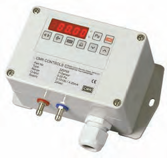
Figure 8: A signal processor that takes the high and low pressure connections (red and blue) and is calibrated to provide direct readings of air flow parameters (Source: CMR Controls)
The pressure signal is typically processed in a local device (such as that shown in Figure 8) that may have a local readout of velocity, pressure difference and volume flow, having been commissioned with the duct dimensions and calibration factor for the measuring device, known as the ‘K factor’ – the airflow required to produce a set value of pressure difference. This is then able to transmit information to the building management system.
© Tim Dwyer, 2014.
References
- Building retuning training guide: AHU minimum outdoor air operation, PNNL–SA–88958, buildingretuning.pnnl.gov/documents/pnnl_sa_88958.pdf , accessed 4 January 2014.
- Legg, R.C., Air-conditioning systems – designing commissioning and maintenance, Batsford, 1991.
- Parsloe, C., BSRIA BG49/2013 Guide to Commissioning Air Systems, BSRIA, 2013.